Statistical Methods and Mapwork

TL;DR

Statistical methods help you analyze geographical data to find patterns and make sense of places, while mapwork focuses on understanding and interpreting maps. Together, these skills let you describe and explain spatial relationships. You'll use calculations, graphs, and map features to uncover geographical insights.

1. The Mental Model

Think of statistical methods as your magnifying glass for geographical numbers, helping you see what's really going on. Mapwork is like reading a story told by lines, colours, and symbols on a map, telling you where things are and why they matter.

2. The Core Material

Geography often involves collecting data (like population numbers, rainfall, or land use) and then making sense of it. That's where statistical methods come in. They help you summarize, analyze, and interpret this data.

2.1 Describing Data: Central Tendency and Dispersion

Photo by RDNE Stock project on Pexels

• Measures of Central Tendency: These tell you about the "average" or typical value in your dataset.
  • Mean: The average (sum all values, then divide by the count).
  • Median: The middle value when data is ordered (if even count, average the two middle ones).
  • Mode: The most frequent value.
• Measures of Dispersion: These tell you how spread out your data is.
  • Range: The difference between the highest and lowest values (Max - Min).
  • Interquartile Range (IQR): The range of the middle 50% of your data (Q3 - Q1), useful for ignoring extreme values.

2.2 Presenting Data

Photo by Kampus Production on Pexels

You can't just list numbers; you need to make them easy to understand.
* Tables: Organize raw or calculated data clearly.
* Graphs: Visual representations are powerful.
* Bar graphs: Compare categories.
* Line graphs: Show trends over time.
* Histograms: Show distribution of continuous data.
* Pie charts: Show proportions of a whole.
* Scatter plots: Show relationships between two variables.

2.3 Mapwork Fundamentals

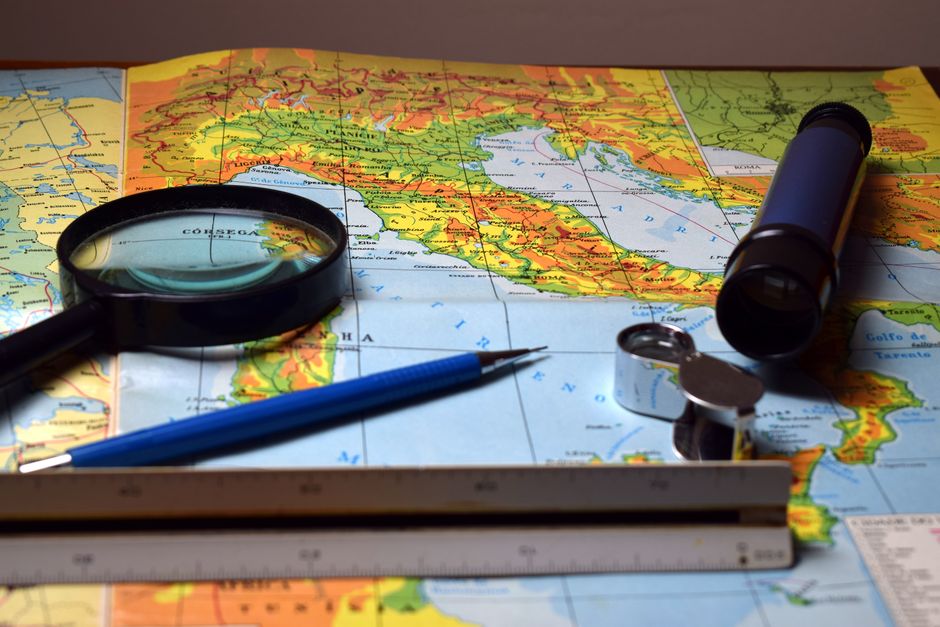
Photo by Ronaldo Guiraldelli on Pexels

Mapwork is about reading, interpreting, and analyzing geographical information presented on maps.

• Scale: The relationship between a distance on the map and the actual distance on the ground.
  • Ratio scale: 1:50 000 (1 unit on map = 50 000 units on ground).
  • Linear scale: A ruler-like line showing distances.
  • Word scale: "1 cm represents 500 meters."
• Direction: Knowing where north is (usually a north arrow).
  • True North: The geographical North Pole.
  • Magnetic North: Where a compass points.
  • Grid North: Parallel to the grid lines on a map.
• Grid References: A system of lines (eastings and northings) to precisely locate points.
  • Four-figure grid reference: Gives a general square (e.g., 2345). You always read Eastings first, then Northings. "Along the corridor, up the stairs."
  • Six-figure grid reference: Pinpoints a location within a square more accurately (e.g., 235452). You estimate 1/10th within the square.
• Contour Lines: Lines on a map joining points of equal elevation above sea level.
  • Closely spaced contours mean a steep slope.
  • Widely spaced contours mean a gentle slope.
  • V-shaped contours point upstream (towards higher elevation).
• Gradient: The steepness of a slope. Calculated as Vertical Interval (VI) / Horizontal Equivalent (HE).
  • VI: The difference in elevation between two points (from contours).
  • HE: The horizontal distance between the two points (measured on map, converted using scale).
• Cross-sections: A profile view showing the changes in elevation along a line on a map.
• Intervisibility: Determining if one point can be seen from another, often by drawing a cross-section.

Here's how map information often leads to statistical analysis:

graph TD
    A["Geographical Phenomenon (e.g., Rainfall)"] --> B["Data Collection (e.g., Rainfall Gauge Readings)"]
    B --> C["Map Plotting (e.g., Isohyet Map)"]
    C --> D["Map Interpretation (e.g., Identify High/Low Rainfall Areas)"]
    D --> E["Statistical Analysis (e.g., Calculate Average Rainfall)"]
    E --> F["Insights & Conclusions (e.g., Relationship between Altitude and Rainfall)"]
    F --> G["Decision Making/Further Research"]

3. Worked Example

Let's calculate the mean and median rainfall for a week, and then find a six-figure grid reference.

Rainfall Data (mm): Monday 12, Tuesday 8, Wednesday 15, Thursday 10, Friday 12, Saturday 20, Sunday 7.

1. Calculate the Mean:
   Sum of values = 12 + 8 + 15 + 10 + 12 + 20 + 7 = 84
   Number of values = 7
   Mean = 84 / 7 = 12 mm

2. Calculate the Median:
   First, order the data: 7, 8, 10, 12, 12, 15, 20
   The middle value (4th out of 7) is 12 mm.

Mapwork Example:
Imagine a map with grid lines. You find a church at the following location:
* It's in the grid square formed by easting line 34 and northing line 67.
* It's about 8/10ths of the way from easting 34 towards 35.
* It's about 3/10ths of the way from northing 67 towards 68.

Your six-figure grid reference would be 348673. (Eastings first: 34, then the 8. Northings second: 67, then the 3.)

4. Key Takeaways

• Central tendency measures (mean, median, mode) describe the "middle" of your data.
• Dispersion measures (range, IQR) show how spread out your data values are.
• Graphs are essential for visualizing patterns and making statistical data easier to understand.
• Map scale is crucial for converting map distances to real-world distances.
• Grid references (eastings then northings) provide precise locations on a map.
• Contour lines show elevation; their spacing indicates the steepness of a slope.
• Gradient quantifies the steepness of a slope using Vertical Interval and Horizontal Equivalent.

Common Mistakes to Avoid:
* Confusing mean, median, and mode; know when to use each one.
* Reading grid references incorrectly (always Eastings first, then Northings).
* Forgetting to convert map distances to real-world distances when using scale.
* Misinterpreting contour line spacing for slope steepness (close = steep, far = gentle).
* Not stating units (e.g., mm, km) for your statistical results or map measurements.

5. Now Try It

Find a local map (digital or physical) that shows contour lines and a grid.
1. Choose three distinct points on the map.
2. Calculate the four-figure and six-figure grid reference for each of your chosen points.
3. For two points that are relatively close but at different elevations, estimate their gradient. You'll need to measure the horizontal distance between them using the map scale and find their vertical interval using contour lines.
4. Success looks like accurately identifying grid references and getting a reasonable gradient calculation, even if you have to estimate the horizontal distance carefully.