Comprehensive Review and Application
From the Bio lab 5 curriculum
TL;DR
This review consolidates the key concepts and experimental techniques you've learned in Bio Lab 5, focusing on how different biological assays work and what their results mean. You'll apply your understanding to interpret experimental outcomes and design new studies. Mastering this involves connecting theory to practical application, ensuring you can troubleshoot experiments and draw valid conclusions.
1. The Mental Model
Think of each lab technique as a specific tool in your biological toolkit. Each tool has a purpose, a set of conditions it works best under, and specific types of data it produces. Your job is to understand when and how to use each tool to answer a biological question.
2. The Core Material
Bio Lab 5 covers a range of essential techniques used to study biological molecules and cellular processes. We've primarily focused on spectrophotometry, protein quantification (Bradford assay), enzyme kinetics, and chromatography.
Spectrophotometry
Spectrophotometry measures how much light a sample absorbs at a specific wavelength. It's fundamental because many biomolecules absorb light (e.g., DNA/RNA at 260 nm, proteins at 280 nm, or specific dyes). The Beer-Lambert Law ($A = \epsilon \cdot l \cdot c$) is key: absorbance ($A$) is directly proportional to the concentration ($c$) of the absorbing substance and the path length ($l$), given the molar absorptivity ($\epsilon$). This allows you to quantify substances by measuring their absorbance.
Protein Quantification (Bradford Assay)
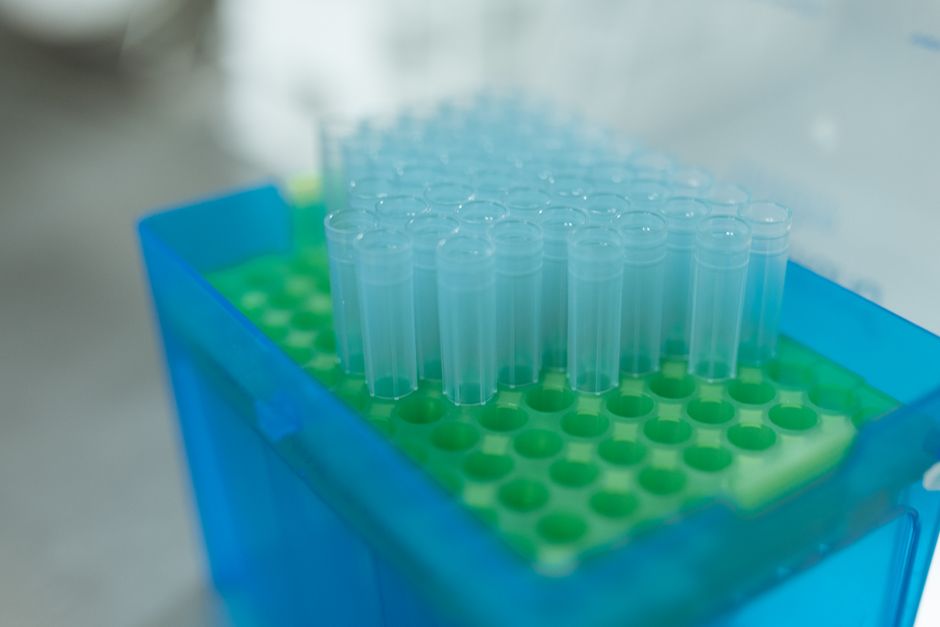
Photo by RDNE Stock project on Pexels
The Bradford assay is a common method to determine protein concentration. It uses Coomassie Brilliant Blue G-250 dye, which binds to basic and aromatic amino acid residues in proteins. When the dye binds, its absorbance maximum shifts from 465 nm (red) to 595 nm (blue). You'll create a standard curve using known protein concentrations (often Bovine Serum Albumin or BSA) to then determine the concentration of unknown samples.
Enzyme Kinetics
Enzyme kinetics studies the rates of enzyme-catalyzed reactions and the factors affecting these rates. Key concepts include:
* Initial reaction rate ($V_0$): The rate at the beginning of the reaction before substrate depletion becomes significant.
* Maximum velocity ($V_{max}$): The maximum rate when the enzyme is saturated with substrate.
* Michaelis constant ($K_m$): The substrate concentration at which the reaction rate is half of $V_{max}$. It reflects the enzyme's affinity for its substrate. A lower $K_m$ means higher affinity.
* Lineweaver-Burk plot: A double reciprocal plot ($1/V_0$ vs. $1/[S]$) that helps determine $V_{max}$ and $K_m$ and differentiate enzyme inhibition types.
Chromatography
Chromatography separates molecules based on their differential distribution between a stationary phase and a mobile phase. We've likely focused on:
* Gel filtration (size exclusion) chromatography: Separates molecules based on size. Larger molecules elute first because they can't enter the pores of the stationary phase beads.
* Ion exchange chromatography: Separates based on charge. The stationary phase has charged groups that bind oppositely charged molecules.
* Affinity chromatography: Separates based on specific binding interactions (e.g., antibody-antigen, enzyme-substrate).
Here's a diagram showing the general workflow for protein quantification using a Bradford assay:
graph TD
    A["Prepare known protein standards"] --> B["Add Bradford reagent to standards and unknowns"];
    B --> C["Incubate (e.g., 5-10 min)"];
    C --> D["Measure absorbance at 595 nm"];
    D --> E["Plot standard curve (Absorbance vs. Conc.)"];
    E --> F["Determine unknown protein concentrations"];
3. Worked Example
Let's say you're given an unknown protein sample and asked to find its concentration using a Bradford assay. You've created a standard curve using BSA. Your standard curve equation is $y = 0.52x + 0.03$, where $y$ is absorbance at 595 nm and $x$ is protein concentration (mg/mL). You measure your unknown sample's absorbance as 0.76.
To find the concentration of your unknown:
$0.76 = 0.52x + 0.03$
$0.76 - 0.03 = 0.52x$
$0.73 = 0.52x$
$x = 0.73 / 0.52$
$x \approx 1.40 \text{ mg/mL}$
So, the concentration of your unknown protein sample is approximately 1.40 mg/mL.
4. Key Takeaways
- Spectrophotometry quantifies substances by measuring light absorption; the Beer-Lambert Law is fundamental.
- Bradford assay uses a dye to quantify proteins, relying on a standard curve generated from known concentrations.
- Enzyme kinetics characterizes enzyme activity using $V_{max}$ and $K_m$, often visualized with Lineweaver-Burk plots.
- Chromatography separates molecules based on physical or chemical properties, using different stationary and mobile phases.
- Understanding the principles behind each technique is crucial for interpreting results and troubleshooting experiments.
- Each technique has specific applications and limitations you need to consider.
- A standard curve is essential for most quantitative assays, allowing you to relate instrument readings to actual concentrations.
Common Mistakes to Avoid:
- Not running appropriate controls (e.g., blanks, positive controls, negative controls) in your experiments.
- Incorrectly interpreting a standard curve, especially extrapolating beyond the linear range.
- Confusing $V_{max}$ with the initial reaction rate, or misinterpreting the significance of $K_m$.
- Failing to account for dilutions when calculating final concentrations.
- Ignoring the importance of pH, temperature, or other reaction conditions on enzyme activity.
5. Now Try It
Imagine you've performed an enzyme kinetics experiment, and you have the following data:
| Substrate Conc. ([S] in mM) | Initial Velocity ($V_0$ in $\mu$mol/min) |
|---|---|
| 0.1 | 10 |
| 0.2 | 18 |
| 0.5 | 30 |
| 1.0 | 40 |
| 2.0 | 45 |
Using this data, prepare a simple Lineweaver-Burk plot (you can sketch it or use a calculator for the reciprocals). Based on your plot, estimate the $V_{max}$ and $K_m$ for this enzyme. What would a competitive inhibitor do to the appearance of this plot?
Success looks like: You've calculated $1/[S]$ and $1/V_0$ values, plotted them to get a rough straight line, estimated where the line crosses the axes (y-intercept for $1/V_{max}$, x-intercept for $-1/K_m$), and can briefly explain how a competitive inhibitor affects the intercepts.
Frequently asked about Comprehensive Review and Application
Study this next
Get the full Bio lab 5 curriculum
Clone the complete plan to your dashboard for unlimited AI-generated notes, practice quizzes, and a personalised revision schedule.
Save this course free