Calculus I: Differentiation and its Applications

TL;DR

Differentiation helps us find the rate at which things change. It's like finding the slope of a curve at any specific point. We'll use it to understand how quantities behave, like finding maximums, minimums, and speeds.

1. The Mental Model

Imagine you're driving a car and want to know your exact speed at a particular moment. Differentiation is the math tool that lets you figure that out, even if your speed is constantly changing. It boils down to finding how steep a curve is at a single point.

2. The Core Material

Differentiation, or finding the derivative, tells us the instantaneous rate of change of a function. Think of it as finding the slope of the tangent line to a curve at a given point. If a function y = f(x) describes a quantity, then its derivative, written as dy/dx or f'(x), describes how y changes with respect to x.

Basic Differentiation Rules

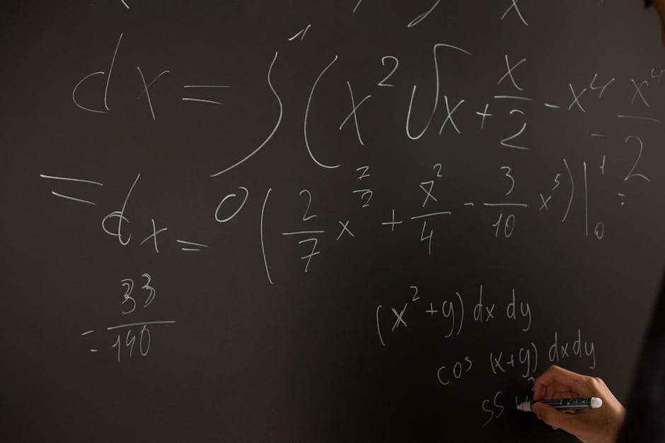
Photo by Monstera Production on Pexels

You'll use these rules constantly:

• Constant Rule: If f(x) = c (where c is a constant), then f'(x) = 0. The rate of change of something that never changes is zero.
  • Example: If f(x) = 5, then f'(x) = 0.
• Power Rule: If f(x) = x^n (where n is any real number), then f'(x) = nx^(n-1). Bring the power down and reduce the power by one.
  • Example: If f(x) = x^3, then f'(x) = 3x^(3-1) = 3x^2.
  • Example: If f(x) = 1/x = x^(-1), then f'(x) = -1x^(-1-1) = -x^(-2) = -1/x^2.
• Constant Multiple Rule: If f(x) = c * g(x), then f'(x) = c * g'(x). You can pull the constant out.
  • Example: If f(x) = 7x^2, then f'(x) = 7 * (2x) = 14x.
• Sum/Difference Rule: If f(x) = g(x) ± h(x), then f'(x) = g'(x) ± h'(x). You can differentiate term by term.
  • Example: If f(x) = x^4 + 3x, then f'(x) = 4x^3 + 3.
• Product Rule: If f(x) = u(x)v(x), then f'(x) = u'(x)v(x) + u(x)v'(x).
  • Example: If f(x) = (x^2)(sin x), u = x^2, v = sin x. u' = 2x, v' = cos x. So f'(x) = (2x)(sin x) + (x^2)(cos x).
• Quotient Rule: If f(x) = u(x)/v(x), then f'(x) = (u'(x)v(x) - u(x)v'(x)) / (v(x))^2. (Low dee high minus high dee low, over low squared).
  • Example: If f(x) = x / (x+1), u = x, v = x+1. u' = 1, v' = 1. So f'(x) = (1(x+1) - x(1)) / (x+1)^2 = (x+1 - x) / (x+1)^2 = 1 / (x+1)^2.
• Chain Rule: If f(x) = g(h(x)), then f'(x) = g'(h(x)) * h'(x). Differentiate the "outer" function, then multiply by the derivative of the "inner" function.
  • Example: If f(x) = (x^2 + 3x)^5. Outer function is ()^5, inner is x^2 + 3x.
  • f'(x) = 5(x^2 + 3x)^4 * (2x + 3).

Applications of Differentiation

Photo by Monstera Production on Pexels

1. Rates of Change: The most direct application. If s(t) is position, s'(t) is velocity, and s''(t) (the second derivative) is acceleration.
2. Tangents and Normals: The derivative f'(a) gives the slope of the tangent line to f(x) at x=a. The slope of the normal line is then -1/f'(a).
3. Optimization (Max/Min problems): To find local maximums or minimums of a function, you set the first derivative f'(x) to zero. These are called critical points. You then use the second derivative test (f''(x)) or the first derivative test to determine if they're maximums or minimums.
   • If f''(x) > 0 at a critical point, it's a local minimum.
   • If f''(x) < 0 at a critical point, it's a local maximum.
4. Increasing/Decreasing Intervals:
   • If f'(x) > 0 on an interval, f(x) is increasing there.
   • If f'(x) < 0 on an interval, f(x) is decreasing there.
5. Concavity and Inflection Points:
   • If f''(x) > 0, f(x) is concave up (like a cup).
   • If f''(x) < 0, f(x) is concave down (like a frown).
   • Inflection points occur where concavity changes, i.e., f''(x) = 0 and f''(x) changes sign.

Here's a flowchart for optimization problems, which are a big deal in applications:

graph TD
    A["Start with problem statement"] --> B["Define function f(x) to optimize"]
    B --> C{"Find f'(x)"}
    C --> D{"Set f'(x) = 0 and solve for x"}
    D --> E["Identify critical points (x values)"]
    E --> F{"Calculate f''(x)"}
    F --> G{{"Evaluate f''(x) at each critical point"}}
    G -- "f''(x) > 0" --> H["Local Minimum"]
    G -- "f''(x) < 0" --> I["Local Maximum"]
    G -- "f''(x) = 0 or undefined" --> J["Second Derivative Test Inconclusive (Use First Derivative Test)"]
    J --> K["Determine global max/min if domain is restricted"]
    K --> L["State conclusion in context of problem"]

3. Worked Example

Let's find the dimensions of a rectangle with perimeter 100 meters that encloses the maximum possible area.

1. Define variables: Let the length be L and the width be W.
2. Formulate equations:
   • Perimeter: 2L + 2W = 100
   • Area: A = L * W
3. Express area as a function of one variable:
   From the perimeter equation, 2L = 100 - 2W, so L = 50 - W.
   Substitute this into the area equation: A(W) = (50 - W) * W = 50W - W^2.
   We want to maximize A(W).
4. Find the derivative:
   A'(W) = d/dW (50W - W^2) = 50 - 2W.
5. Set derivative to zero to find critical points:
   50 - 2W = 0
2W = 50
W = 25
6. Use the second derivative test to confirm it's a maximum:
   A''(W) = d/dW (50 - 2W) = -2.
   Since A''(25) = -2 (which is less than 0), this confirms that W = 25 corresponds to a local maximum.
7. Find the other dimension:
   If W = 25, then L = 50 - 25 = 25.
8. Conclusion: The rectangle with the maximum area for a perimeter of 100 meters is a square with sides of 25 meters. The maximum area is 25 * 25 = 625 square meters.

4. Key Takeaways

• Differentiation measures the instantaneous rate of change or the slope of a tangent line.
• The power rule, product rule, quotient rule, and chain rule are essential for finding derivatives.
• Setting the first derivative to zero helps find critical points, which are potential maximums or minimums.
• The second derivative test helps distinguish between local maximums (negative second derivative) and local minimums (positive second derivative).
• If the first derivative is positive, the function is increasing; if negative, it's decreasing.
• If the second derivative is positive, the function is concave up; if negative, it's concave down.

Common Mistakes to Avoid:
- Forgetting the Chain Rule, especially with functions like sin(2x) or (x^2+1)^3.
- Mixing up the Product and Quotient Rules (remember "low dee high minus high dee low...").
- Incorrectly simplifying after differentiation, particularly with negative exponents.
- Not checking the second derivative for max/min problems – a critical point might be an inflection point.
- Forgetting to answer the original question in optimization problems (e.g., finding just x instead of the actual dimensions or maximum value).

5. Now Try It

A particle's position (in meters) along an axis is given by s(t) = t^3 - 6t^2 + 9t, where t is time in seconds, for 0 <= t <= 5.

1. Find the particle's velocity function, v(t).
2. Find the particle's acceleration function, a(t).
3. Determine the time intervals when the particle is moving to the right (i.e., when its velocity is positive).
4. Find