Linear Equations and Their Graphs

TL;DR

Linear equations describe a straight line on a graph, showing a consistent relationship between two variables. You'll learn to recognize, manipulate, and plot these equations to visualize that relationship. Understanding them is fundamental for modeling many real-world scenarios in applied math.

1. The Mental Model

Think of a linear equation as a recipe for a straight line. It tells you exactly how much one thing changes when another thing changes, always at the same steady rate. Graphing it lets you "see" that relationship instantly.

2. The Core Material

A linear equation typically involves two variables, often x and y, and when you plot all the possible pairs of (x, y) that satisfy the equation, they form a straight line. The most common form you'll encounter is the slope-intercept form:

y = mx + b

Let's break down what each part means:

• y: This is your dependent variable. Its value depends on x.
• x: This is your independent variable. You can choose any value for x, and it will determine y.
• m: This is the slope of the line. It tells you how steep the line is and its direction.
  • A positive m means the line goes up from left to right.
  • A negative m means the line goes down from left to right.
  • m is calculated as "rise over run" – the change in y divided by the change in x between any two points on the line.
• b: This is the y-intercept. It's the point where the line crosses the y-axis (meaning x = 0).

Graphing a Linear Equation

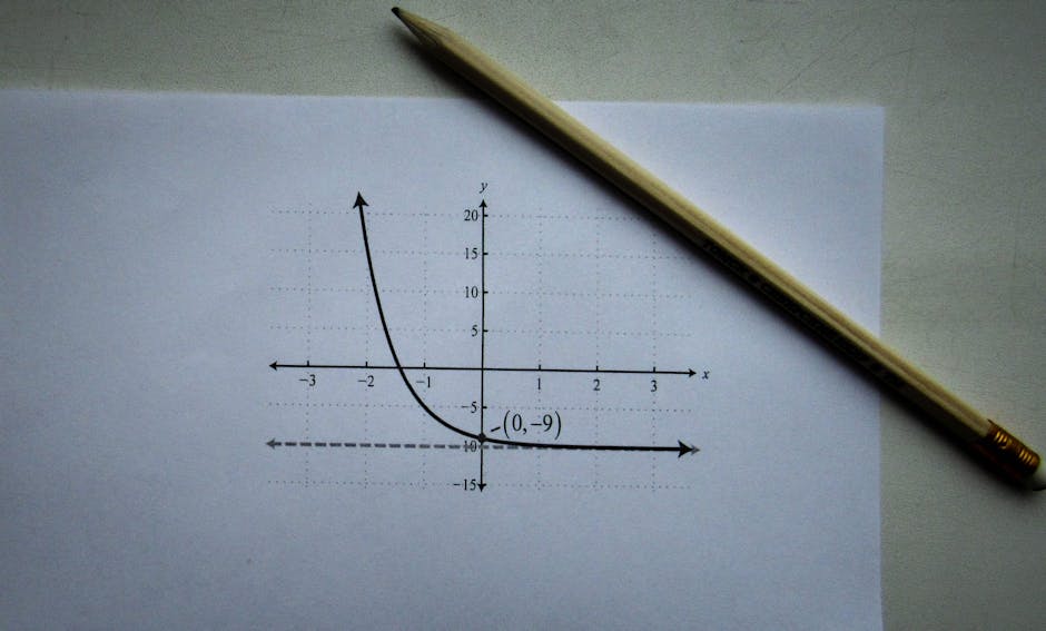
Photo by Sergey Meshkov on Pexels

To graph a linear equation, you generally need two points. The easiest points to find are often the intercepts.

a. Using the Slope and Y-intercept

This is often the quickest way if your equation is already in y = mx + b form.

1. Plot the y-intercept (b): This is your starting point on the y-axis.
2. Use the slope (m) to find a second point: Remember m = rise / run. From your y-intercept, count "up" (or down if negative) by the rise amount, then "right" (or left if negative) by the run amount. Plot this second point.
3. Draw the line: Connect the two points and extend the line with arrows on both ends to show it continues infinitely.

b. Using Two Points (e.g., x- and y-intercepts)

If the equation isn't easily in y = mx + b form, or you prefer this method:

1. Find the y-intercept: Set x = 0 and solve for y. This gives you the point (0, y).
2. Find the x-intercept: Set y = 0 and solve for x. This gives you the point (x, 0).
3. Plot both intercepts and draw the line connecting them.

Different Forms of Linear Equations

Photo by Monstera Production on Pexels

While y = mx + b is super useful for graphing, you might see other forms:

• Standard Form: Ax + By = C (where A, B, and C are constants). This is often good for finding intercepts quickly.
• Point-Slope Form: y - y1 = m(x - x1) (where (x1, y1) is a known point on the line). This is handy if you know a point and the slope.

The Relationship Between Slope, Y-Intercept, and the Graph

Photo by Sergey Meshkov on Pexels

graph TD
    Start["Linear Equation (e.g., y = mx + b)"] --> IdentifySlope["Identify Slope (m)"]
    Start --> IdentifyYIntercept["Identify Y-Intercept (b)"]

    IdentifyYIntercept --> PlotYIntercept["Plot Point (0, b) on y-axis"]
    IdentifySlope --> DetermineDirection["Determine Direction:
        m > 0 (Upward / Right)
        m < 0 (Downward / Right)
        m = 0 (Horizontal)"]
    IdentifySlope --> DetermineSteepness["Determine Steepness:
        Large |m| -> Steeper
        Small |m| -> Flatter"]

    PlotYIntercept --> UseSlope["From (0, b), use 'rise/run' of m"]
    UseSlope --> FindSecondPoint["Find a Second Point (x_new, y_new)"]
    FindSecondPoint --> DrawLine["Draw Straight Line through both points"]

3. Worked Example

Let's graph the equation 2x + 3y = 6.

First, let's convert it to slope-intercept form (y = mx + b) to make graphing easier.

1. Isolate the y term:
   3y = -2x + 6

2. Divide by 3:
   y = (-2/3)x + 2

Now we have m = -2/3 and b = 2.

• Step 1: Plot the y-intercept.
  Since b = 2, the line crosses the y-axis at (0, 2). Plot this point.

• Step 2: Use the slope to find another point.
  The slope m = -2/3 means "rise = -2" and "run = 3".
  From our y-intercept (0, 2):

  • Go down 2 units (because rise is -2). This puts us at y = 0.
  • Go right 3 units (because run is 3). This puts us at x = 3.
  • So, our second point is (3, 0).

• Step 3: Draw the line.
  Connect the point (0, 2) and (3, 0) with a straight line, extending it with arrows.

You could also find the x-intercept directly:
Set y = 0 in 2x + 3y = 6:
2x + 3(0) = 6
2x = 6
x = 3
So the x-intercept is (3, 0), which matches the second point we found using the slope!

4. Key Takeaways

• A linear equation always graphs as a straight line, representing a constant rate of change.
• The slope (m) tells you the steepness and direction of the line ("rise over run").
• The y-intercept (b) is where the line crosses the y-axis (when x = 0).
• The most useful form for graphing is y = mx + b.
• You only need two points to draw a unique straight line.
• Plotting the y-intercept and then using the slope is a fast way to graph.

Common Mistakes to Avoid:
- Mixing up rise and run: always rise (change in y) over run (change in x).
- Incorrectly handling negative signs in the slope or when solving for intercepts.
- Thinking y = mx is different; it's just y = mx + 0, so the y-intercept is (0,0).
- Forgetting to extend the line with arrows, implying it stops at your plotted points.

5. Now Try It

Graph the linear equation y = (1/2)x - 3. First, identify the slope and y-intercept. Then, plot the y-intercept and use the slope to find a second point. Finally, draw the line. Success looks like a straight line that passes through (0, -3) and (2, -2).