Applications in Open Channel Flow and Hydraulic Structures

TL;DR

You'll learn how the Navier-Stokes equations simplify into the equations engineers actually use for rivers, canals, and spillways. You'll see how depth-averaging turns a 3D problem into the Saint-Venant equations, and how these predict flow over weirs, through hydraulic jumps, and under gates. You'll also understand why the Froude number, not Reynolds number, dominates channel design decisions.

1. The Mental Model

Open channel flow is Navier-Stokes with one boundary that's free to move: the water surface. Gravity drives the flow instead of a pump, and pressure at the surface is always atmospheric. Because channels are usually much longer than they are deep, engineers average the equations over depth instead of solving every vertical layer. The core idea: open channel hydraulics is Navier-Stokes flattened by gravity and simplified by geometry.

2. The Core Material

From Navier-Stokes to Saint-Venant

Photo by Erik Mclean on Pexels

Start with the full incompressible Navier-Stokes equations:

$$\rho\left(\frac{\partial \mathbf{u}}{\partial t} + \mathbf{u}\cdot\nabla\mathbf{u}\right) = -\nabla p + \mu\nabla^2\mathbf{u} + \rho\mathbf{g}$$

For a river or canal, three simplifications matter. First, the flow is shallow: depth $h$ is tiny compared to length $L$, so vertical acceleration is negligible and pressure becomes hydrostatic, $p = \rho g(h-z)$. Second, velocity is nearly uniform across the cross-section, so you can replace the full velocity field with a depth-averaged value $V$. Third, friction against the bed replaces viscous stress as the dominant resistance term, since turbulence — not molecular viscosity — controls momentum loss in real channels.

Applying these to the x-momentum equation and integrating over depth gives the Saint-Venant equations — the open-channel flow workhorse:

Continuity (mass conservation):
$$\frac{\partial A}{\partial t} + \frac{\partial Q}{\partial x} = 0$$

Momentum:
$$\frac{\partial Q}{\partial t} + \frac{\partial}{\partial x}\left(\frac{Q^2}{A}\right) + gA\frac{\partial h}{\partial x} = gA(S_0 - S_f)$$

Here $A$ is cross-sectional area, $Q$ is discharge, $S_0$ is the bed slope, and $S_f$ is the friction slope (from something like Manning's equation). Notice what happened: the viscous term $\mu\nabla^2\mathbf{u}$ got replaced by $S_f$, an empirical friction term, because turbulent boundary layers near a rough channel bed aren't well captured by molecular viscosity alone. This is the price of depth-averaging — you trade exact physics for a workable 1D model, and you patch the gap with empirical closure relations like Manning's $n$.

The Froude Number and Flow Regimes

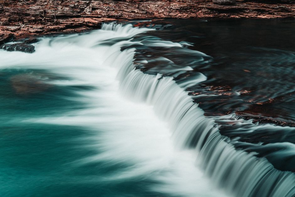
Photo by Connor Scott McManus on Pexels

In pipe flow, Reynolds number tells you laminar versus turbulent. In open channels, the number that governs behavior is the Froude number:

$$Fr = \frac{V}{\sqrt{gh}}$$

This compares flow velocity to the speed of a surface gravity wave, $\sqrt{gh}$. When $Fr < 1$ (subcritical), disturbances can travel upstream — a downstream obstruction (like a weir) affects flow upstream of it. When $Fr > 1$ (supercritical), disturbances can't propagate upstream — the flow is too fast, and waves just wash downstream. When $Fr = 1$, you're at critical flow, where a unique relationship exists between depth and discharge for a given channel shape.

This matters enormously for structures. A sluice gate accelerates flow from subcritical to supercritical. A hydraulic jump does the reverse — it's the abrupt, turbulent transition where supercritical flow slams back to subcritical, dissipating huge amounts of kinetic energy as heat and turbulence. You see this every time water leaves a spillway and churns violently at the base.

flowchart TD
    A["Reservoir: still water, high energy"] --> B["Spillway crest: flow accelerates, Fr < 1"]
    B --> C["Spillway face: supercritical flow, Fr > 1"]
    C --> D["Stilling basin: hydraulic jump"]
    D --> E["Downstream channel: subcritical flow, Fr < 1"]
    D --> F["Energy dissipated as turbulence and heat"]

Applying This to Hydraulic Structures

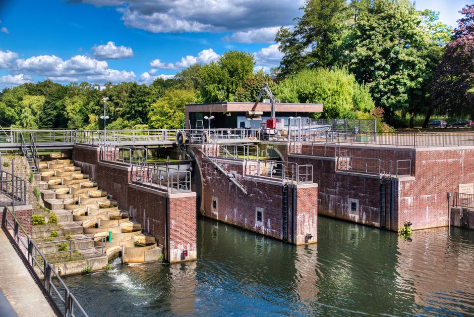
Photo by Paparazzi Ratzfatzzi on Pexels

Weirs. A weir is a controlled obstruction that forces critical flow over its crest, which is why weirs are used as flow-measurement devices — once you're at critical depth, discharge depends only on upstream head $H$:

$$Q = C_d \, L \, \sqrt{g}\, H^{3/2}$$

where $L$ is crest length and $C_d$ is a discharge coefficient absorbing all the messy 3D effects (contraction, viscosity, surface tension) that the simple 1D model ignores.

Sluice gates. These control discharge by throttling the opening. Applying the Bernoulli equation (a special case of Navier-Stokes when viscous and unsteady terms vanish) between upstream still water and the vena contracta downstream gives:

$$Q = C_d \, b \, a \, \sqrt{2g(H-a)}$$

where $b$ is gate width, $a$ is the gate opening, and $H$ is upstream head. The flow downstream of the gate is supercritical — fast and shallow — setting up the conditions for a hydraulic jump further downstream.

Hydraulic jumps and stilling basins. Using the momentum equation across the jump (not Bernoulli, because energy is lost) gives the depth ratio for a jump in a rectangular channel:

$$\frac{h_2}{h_1} = \frac{1}{2}\left(\sqrt{1+8Fr_1^2}-1\right)$$

Engineers design stilling basins specifically to force this jump to happen in a controlled, armored location instead of letting it erode the unprotected riverbed downstream.

Continue with the Worked Example below.

3. Worked Example

Problem: A rectangular spillway channel is 4 m wide. Water flows under a sluice gate with an opening $a = 0.5$ m, upstream head $H = 3.0$ m, and discharge coefficient $C_d = 0.6$. Find the discharge, the downstream depth, and check whether a hydraulic jump will form — then find the jump's downstream depth.

Step 1: Discharge through the gate.

$$Q = C_d \, b \, a \, \sqrt{2g(H-a)}$$
$$Q = 0.6 \times 4 \times 0.5 \times \sqrt{2 \times 9.81 \times (3.0-0.5)}$$
$$Q = 1.2 \times \sqrt{49.05} = 1.2 \times 7.00 = 8.40\ \text{m}^3/\text{s}$$

Step 2: Depth just downstream of the gate (vena contracta).

Assume the contraction coefficient makes the effective depth $h_1 \approx 0.6 \times a = 0.3$ m (a standard approximation for sharp gates).

Check velocity:
$$V_1 = \frac{Q}{b \, h_1} = \frac{8.40}{4 \times 0.3} = 7.0\ \text{m/s}$$

Step 3: Froude number at $h_1$.

$$Fr_1 = \frac{V_1}{\sqrt{g h_1}} = \frac{7.0}{\sqrt{9.81 \times 0.3}} = \frac{7.0}{1.72} = 4.08$$

Since $Fr_1 = 4.08 \gg 1$, the flow is strongly supercritical right after the gate — exactly what you'd expect. This sets up conditions for a hydraulic jump downstream if the channel's normal (subcritical) depth is imposed by a control further along (say, a weir or the natural channel slope).

Step 4: Sequent depth after the jump.

$$\frac{h_2}{h_1} = \frac{1}{2}\left(\sqrt{1+8(4.08)^2}-1\right) = \frac{1}{2}\left(\sqrt{1+133.1}-1\right) = \frac{1}{2}(11.58-1) = 5.29$$

$$h_2 = 5.29 \times 0.3 = 1.59\ \text{m}$$

Step 5: Sanity check with velocity and Froude number after the jump.

$$V_2 = \frac{Q}{b\,h_2} = \frac{8.40}{4 \times 1.59} = 1.32\ \text{m/s}$$
$$Fr_2 = \frac{1.32}{\sqrt{9.81 \times 1.59}} = \frac{1.32}{3.95} = 0.33$$

$Fr_2 = 0.33 < 1$ confirms the flow is now subcritical — the jump did