Applications in Pipe Networks, Pumps, and Water Distribution Systems

TL;DR

You'll learn how the Navier-Stokes equations collapse into the practical head-loss and energy-balance tools engineers actually use to size pipes and pumps. You'll see how Darcy-Weisbach and the Hazen-Williams equation come from the same physics as full N-S, just heavily simplified for steady pipe flow. You'll finish able to solve a real pump-pipe system problem by hand.

1. The Mental Model

Full Navier-Stokes tracks every swirl and stress in a fluid, but a pipe forces the flow into one direction, so almost all of that complexity disappears. What's left is a balance sheet: energy in from a pump equals energy lost to friction plus energy needed to lift or accelerate the water. Every pipe network problem is really just "where does the energy go?" asked over and over at every junction. A pipe network is Navier-Stokes reduced to bookkeeping of energy along one-dimensional flow paths.

2. The Core Material

From Navier-Stokes to the Pipe Flow Equation

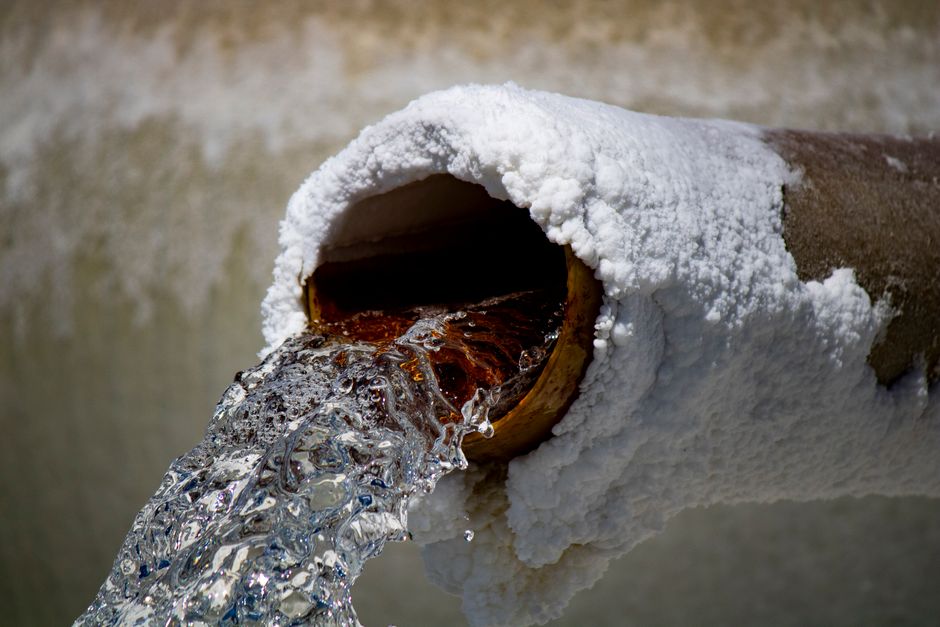
Photo by Orhan Akbaba on Pexels

The full incompressible Navier-Stokes equation is:

$$\rho\left(\frac{\partial \vec{v}}{\partial t} + \vec{v}\cdot\nabla \vec{v}\right) = -\nabla p + \mu \nabla^2 \vec{v} + \rho \vec{g}$$

In a straight pipe, three simplifications gut this equation down to something usable. First, flow is fully developed and axial, so the velocity only has one component and it only varies with radial position, not along the pipe's length (except for the pressure driving it). Second, for steady flow the time-derivative term vanishes. Third, gravity acts only along the pipe's axis if the pipe is tilted, which is handled separately as elevation head.

What survives, for laminar flow, is a balance between the pressure gradient and viscous shear:

$$0 = -\frac{dp}{dx} + \mu \frac{1}{r}\frac{d}{dr}\left(r\frac{dv_x}{dr}\right)$$

Solving this with a no-slip condition at the pipe wall gives the parabolic Hagen-Poiseuille velocity profile, and integrating that over the pipe's cross-section gives the famous laminar flow relation:

$$\Delta p = \frac{128 \mu L Q}{\pi D^4}$$

This is exact — a genuine analytical solution of Navier-Stokes. But almost all real pipe flow in water systems is turbulent (Reynolds number in the thousands to millions), and turbulence means you cannot solve N-S analytically anymore. Turbulent eddies mix momentum in ways no closed-form solution captures. So engineers replace the viscous term with an empirical friction factor, giving the Darcy-Weisbach equation:

$$h_f = f \frac{L}{D}\frac{v^2}{2g}$$

Here $h_f$ is head loss (in meters of water), $f$ is the Darcy friction factor (found from the Moody chart or the Colebrook equation, which depends on Reynolds number and pipe roughness), $L$ is pipe length, $D$ is diameter, and $v$ is mean velocity. This equation is derived from the same momentum balance as N-S but with $f$ absorbing all the turbulent chaos empirically — this is exactly the same trick used in Reynolds-Averaged Navier-Stokes (RANS) modeling, just algebraically packaged for a pipe.

A simpler empirical alternative widely used in water distribution design is Hazen-Williams:

$$v = 0.849\, C_{HW}\, R_h^{0.63} S^{0.54}$$

where $C_{HW}$ is a roughness coefficient (around 100-150 for typical pipes), $R_h$ is the hydraulic radius, and $S$ is the slope of the energy grade line. It's less physically rigorous than Darcy-Weisbach but faster to use and standard in US water utility work.

Energy Balance with Pumps: The Extended Bernoulli Equation

Photo by Markus Winkler on Pexels

Real pipe networks include pumps, so the steady-flow energy equation (Bernoulli extended with losses and pump work) governs system design:

$$\frac{p_1}{\rho g} + \frac{v_1^2}{2g} + z_1 + h_{pump} = \frac{p_2}{\rho g} + \frac{v_2^2}{2g} + z_2 + h_f + h_{minor}$$

Every term here is an energy per unit weight of fluid (units of length, called "head"). $h_{pump}$ is energy added by the pump, $h_f$ is friction loss from Darcy-Weisbach, and $h_{minor}$ covers losses from fittings, valves, and bends (each modeled as $K \frac{v^2}{2g}$ with a loss coefficient $K$).

The pump itself has a characteristic curve: it delivers less head as flow rate increases, typically modeled as

$$h_{pump} = a - bQ^2$$

The system curve is the pipe's demand: head required rises with flow squared because friction loss scales with $v^2$:

$$h_{system} = h_{static} + kQ^2$$

The operating point is where these two curves intersect — where the pump's supply matches the pipe's demand exactly.

graph TD
    A["Pump adds energy: h_pump = a - bQ²"] --> B["Flow enters pipe network"]
    B --> C["Friction loss along pipes: h_f = f (L/D)(v²/2g)"]
    B --> D["Minor losses at fittings/valves: h_minor = K(v²/2g)"]
    C --> E["Elevation change: z2 - z1"]
    D --> E
    E --> F["System curve: h_system = h_static + kQ²"]
    A --> G["Operating point: intersection of pump curve and system curve"]
    F --> G

Networks: Continuity at Junctions and the Hardy Cross Method

Photo by Cheng on Pexels

Real water distribution systems aren't single pipes — they're loops and branches. Two physical laws from the underlying conservation equations govern them, mirroring mass and momentum conservation in full N-S:

1. Continuity at nodes: flow in equals flow out at every junction (mass conservation, exactly like $\nabla \cdot \vec{v} = 0$ for incompressible flow, just applied at discrete points).
2. Energy conservation around loops: the sum of head losses around any closed loop must equal zero.

Because head loss is nonlinear in flow ($h_f \propto Q^{1.85}$ to $Q^2$ depending on the formula used), you can't solve networks with simple linear algebra. The classic hand method is the Hardy Cross method: guess an initial flow distribution, compute the loop imbalance, and iteratively correct flows using a correction formula until loops balance. Modern software (EPANET, WaterCAD) does this same relaxation numerically, but the physics is identical — it's Newton-Raphson-style iteration applied to nonlinear energy balance equations.

3. Worked Example

A pump must move water from a reservoir at elevation 10 m to a tank at elevation 45 m through a single steel pipe, 500 m long, with an internal diameter of 0.3 m. The friction factor is $f = 0.02$ (typical for this Reynolds number and roughness). Minor losses total $K = 5$ (combined valves and bends). Find the required pump head when the desired flow rate is $Q = 0.15\, \text{m}^3/\text{s}$, and check what pump head is needed at that flow.

Step 1: velocity in the pipe.

$$A = \frac{\pi D^2}{4} = \frac{\pi (0.3)^2}{4} = 0.0707\, \text{m}^2$$

$$v = \frac{Q}{A} = \frac{0.15}{0.0707} = 2.12\, \text{m/s}$$

Step 2: friction loss (Darcy-Weisbach).

$$h_f = f\frac{L}{D}\frac{v^2}{2g} = 0.02 \times \frac{500}{0.3} \times \frac{(2.12)^2}{2(9.81)}$$

$$h_f = 0.02 \times 1666.7 \times 0.229 = 7.63\, \text{m}$$

Step 3: minor losses.

$$h_{minor} = K\frac{v^2}{2g} = 5 \times \frac{(2.12)^2}{2(9.81)} = 5 \times 0.229 = 1.15\, \text{m}$$

Step 4: elevation (static) head.

$$h_{static} = z_2 - z_1 = 45 - 10 = 35\, \text{m}$$

Step 5: total pump head required.

$$h_{pump} = h_{static} + h_f + h_{minor} = 35 + 7.63 + 1.15 = 43.78\, \text{m}$$

So the pump must supply about 43.8 m of head at $Q = 0.15\, \text{m}^3/\text{s}$ for the system to deliver that flow. If the manufacturer's pump curve is