Introduction to Linear Functions

TL;DR

Linear functions describe a straight line relationship between two variables, where a change in one variable causes a proportional change in the other. They are represented by the equation y = mx + b, where 'm' is the slope and 'b' is the y-intercept. Understanding these functions helps predict outcomes and model real-world scenarios.

1. The Mental Model

Imagine you're driving at a constant speed. The further you drive, the more distance you cover in a perfectly predictable way. A linear function is like that constant speed, showing how one thing changes consistently in response to another.

2. The Core Material

A linear function shows a relationship where the output changes at a constant rate for every unit change in the input. When you plot this relationship on a graph, it always forms a straight line.

The most common form of a linear function is called the slope-intercept form:

y = mx + b

Let's break down what each part means:

• y: This is your dependent variable (the output). Its value depends on the value of x.
• x: This is your independent variable (the input). You choose its value, and it affects y.
• m: This is the slope of the line. It tells you how steep the line is and in what direction (up or down).
  • A positive m means the line goes up from left to right.
  • A negative m means the line goes down from left to right.
  • m is the "rate of change" – how much y changes for every 1 unit change in x. You can calculate it as "rise over run": m = (change in y) / (change in x).
• b: This is the y-intercept. It's the point where the line crosses the y-axis (the vertical axis). At this point, the value of x is always 0. It's often the starting value or a fixed cost.

Graphing a Linear Function

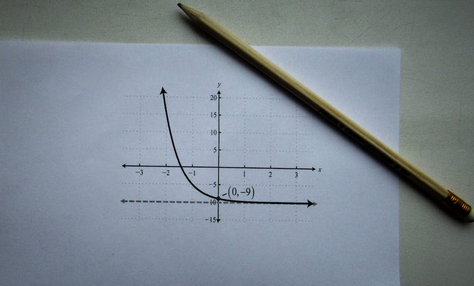
Photo by Sergey Meshkov on Pexels

To graph a linear function, you typically need two points. The y-intercept (b) gives you one easy point (0, b). From there, you can use the slope (m) to find another point.

graph TD
    A["Start with the Equation: y = mx + b"] --> B["Identify 'b' (y-intercept)"];
    B --> C["Plot the y-intercept (0, b) on the y-axis"];
    C --> D{"Is 'm' (slope) positive or negative?"};
    D -- "Positive 'm'" --> E["Move 'm' units UP for 'rise'"];
    D -- "Negative 'm'" --> F["Move 'm' units DOWN for 'rise'"];
    E --> G["Then move 1 unit RIGHT for 'run'"];
    F --> G;
    G --> H["Plot the new point"];
    H --> I["Draw a straight line through both points"];

3. Worked Example

Let's work with the linear function: y = 2x + 3.

1. Identify m and b:

   • m (slope) = 2
   • b (y-intercept) = 3

2. Plot the y-intercept: This is the point (0, b). So, plot a point at (0, 3) on your graph.

3. Use the slope to find another point:

   • The slope m = 2 can be written as 2/1. This means for every 1 unit you move to the right on the x-axis, you move 2 units up on the y-axis.
   • Starting from your y-intercept (0, 3):
     • Move 1 unit to the right (x goes from 0 to 1).
     • Move 2 units up (y goes from 3 to 5).
   • This gives you a new point: (1, 5).

4. Draw the line: Connect the point (0, 3) and (1, 5) with a straight line. This line represents the function y = 2x + 3.

4. Key Takeaways

• A linear function always produces a straight line when graphed.
• The equation y = mx + b is the standard slope-intercept form for a linear function.
• m represents the slope, which is the constant rate of change of y with respect to x.
• b represents the y-intercept, the point where the line crosses the y-axis (where x = 0).
• You only need two points to draw a unique straight line.
• Linear functions are used to model situations with a constant rate of change, like costs over time or distance traveled.

Common Mistakes to Avoid

Photo by KATRIN BOLOVTSOVA on Pexels

• Confusing m and b: Remember m affects the steepness/direction, b affects where it starts on the y-axis.
• Incorrectly plotting the y-intercept: It's always (0, b), not (b, 0).
• Misinterpreting the slope: If m is a whole number (e.g., 3), remember it's 3/1 (rise of 3, run of 1). If it's a fraction like 1/2, it's a rise of 1 for a run of 2.
• Drawing a curve: Linear functions are always straight lines. If your graph isn't straight, you've made a mistake.

5. Now Try It

Take the function y = -1/2x + 4.
1. Identify its slope (m) and y-intercept (b).
2. Plot the y-intercept on a piece of graph paper.
3. Use the slope to find a second point.
4. Draw the line.

Success looks like: You have a straight line that crosses the y-axis at y=4 and goes downwards from left to right, with a gentle slope (down 1 unit for every 2 units right).