Standard Curve Preparation and Measurement Protocol

TL;DR

A standard curve uses known concentrations of a substance to create a visual representation that helps you determine unknown concentrations in samples. You prepare a series of dilutions from a stock solution, measure their absorbances, and plot these points to create a calibration line. This line allows you to accurately interpolate the concentration of your experimental samples based on their measured absorbance.

1. The Mental Model

Imagine you have a ruler (your standard curve) where you know exactly what each mark means (known concentrations). When you measure something unknown (your sample), you can place it against your ruler and figure out its value.

2. The Core Material

Preparing a standard curve is crucial for many lab assays, especially those relying on spectrophotometry (measuring light absorption). It establishes a relationship between the concentration of a substance and the signal you're measuring (e.g., absorbance).

2.1 Preparing the Stock Solution

Photo by Mikhail Nilov on Pexels

First, you need a stock solution of your analyte (the substance you're trying to measure) at a known, high concentration.
* Dissolve a precisely weighed amount of pure analyte in a known volume of solvent.
* Calculate the exact concentration (e.g., in mg/mL, µM). This will be your starting point for dilutions.

2.2 Creating a Dilution Series

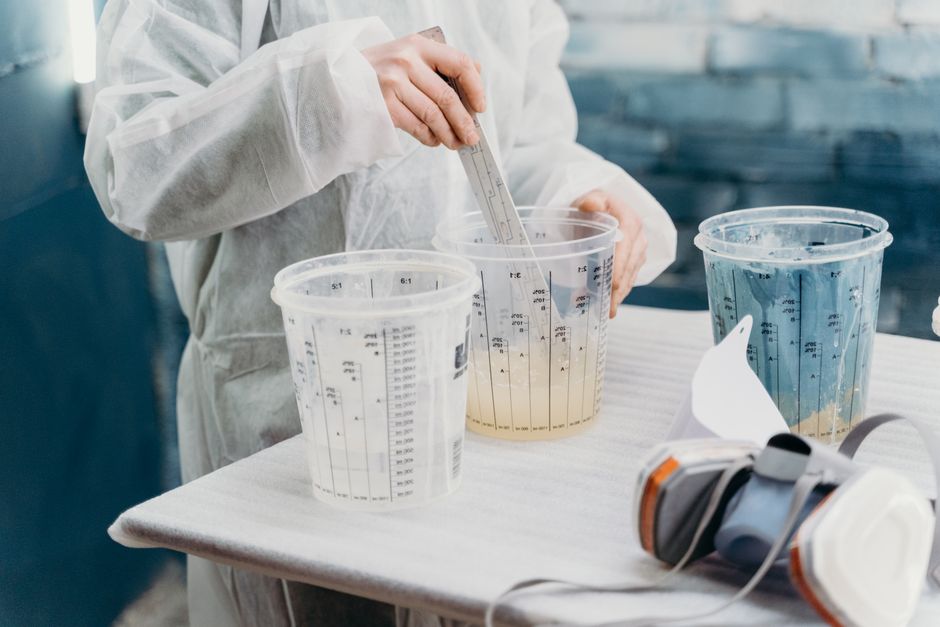
Photo by cottonbro studio on Pexels

You'll prepare several tubes or wells, each containing a different, known concentration of your analyte. These are your "standards."
* Serial Dilution: This is often the most efficient way. You start with your stock solution and dilute it step-by-step. For example, to make a 1:2 dilution series:
1. Take a portion of your stock solution (e.g., 500 µL) into the first tube. This is your highest standard concentration.
2. Add an equal volume of diluent (e.g., 500 µL water or buffer) to the next tube.
3. Transfer 500 µL from the first tube to the second tube. Mix well. This tube now has half the concentration of the first.
4. Repeat the transfer process from the second tube to the third, and so on, until you have your desired range of concentrations.
* Independent Dilution: Less common for a full series, but sometimes used. You calculate the exact volume of stock needed for each specific standard concentration and dilute it directly into its final volume. This can be more precise but more time-consuming for many points.
* Always include a blank (0 concentration) containing only your diluent. This accounts for any background signal from the reagents or solvent itself.

2.3 Measuring Absorbance (or other signal)

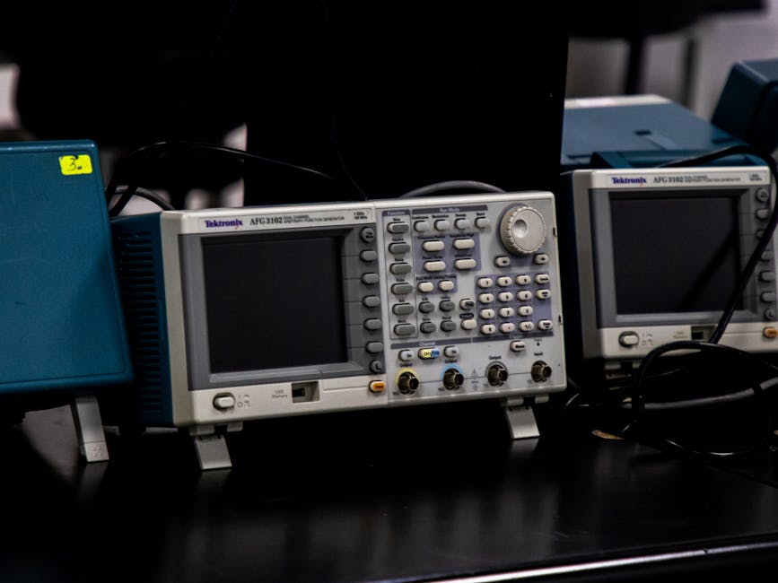
Photo by Ludovic Delot on Pexels

Once your standards are prepared, you'll measure their absorbance (or fluorescence, color intensity, etc.) using the appropriate instrument (e.g., spectrophotometer, plate reader).
* Ensure your instrument is properly calibrated and warmed up.
* Set the correct wavelength for your assay.
* Measure the absorbance of your blank first, then each of your standards, usually from lowest to highest concentration to minimize carryover.
* Record all measurements carefully.

2.4 Plotting the Standard Curve

Photo by Tara Winstead on Pexels

You'll plot your data to visualize the relationship between concentration and absorbance.
* X-axis: Concentration of the analyte (independent variable).
* Y-axis: Absorbance (dependent variable).
* Plot each (concentration, absorbance) pair.
* Draw a line of best fit through these points. For many assays, this will be a straight line (linear regression).
* The equation of this line (y = mx + c) is what you'll use for calculations.

graph TD
    A["Prepare Stock Solution (Known High Conc.)"] --> B["Create Dilution Series (Known Concentrations)"];
    B --> C["Prepare Blank (0 Conc.)"];
    C --> D["Measure Absorbance of Blank"];
    D --> E["Measure Absorbance of Standards (Lowest to Highest)"];
    E --> F["Record All Absorbance Values"];
    F --> G["Plot Concentration vs. Absorbance"];
    G --> H["Perform Linear Regression (Get y=mx+c)"];
    H --> I["Measure Absorbance of Unknown Samples"];
    I --> J["Use Standard Curve Equation to Find Unknown Concentrations"];

2.5 Measuring Unknown Samples

Once your standard curve is established:
* Prepare your experimental samples using the same reagents and protocol as your standards (except you don't know their concentration yet).
* Measure their absorbance using the exact same instrument settings.
* Use the equation of your standard curve (y = mx + c, where y is absorbance and x is concentration) to calculate the concentration of your unknown samples.
* Concentration (x) = (Absorbance (y) - c) / m

3. Worked Example

Let's say you're measuring protein concentration using a Bradford assay, and your standard protein is Bovine Serum Albumin (BSA).

1. Stock Solution: You prepare a 2.0 mg/mL BSA stock solution.
2. Dilution Series: You decide on standards of 0, 0.1, 0.25, 0.5, 0.75, and 1.0 mg/mL.
   • You'd calculate how much 2.0 mg/mL stock and diluent (e.g., water) you need for each. For example, to make 500 µL of 1.0 mg/mL: (C1V1 = C2V2) -> (2.0 mg/mL * V1 = 1.0 mg/mL * 500 µL) -> V1 = 250 µL. So, 250 µL of stock + 250 µL of water.
   • The 0 mg/mL standard is just 500 µL of water (your blank).
3. Assay & Measurement: You add Bradford reagent to each standard and let it incubate. Then, you measure absorbance at 595 nm using a spectrophotometer.
   • Blank (0 mg/mL): 0.050
   • 0.1 mg/mL: 0.120
   • 0.25 mg/mL: 0.280
   • 0.5 mg/mL: 0.520
   • 0.75 mg/mL: 0.770
   • 1.0 mg/mL: 1.010
4. Plotting: You plot these points in Excel or similar software. You perform a linear regression. Let's say the software gives you the equation: y = 0.985x + 0.045 (where y is absorbance and x is concentration).
5. Unknown Sample: You run an unknown sample and its absorbance at 595 nm is 0.650.
   • Using the equation: 0.650 = 0.985x + 0.045
   • 0.650 - 0.045 = 0.985x
   • 0.605 = 0.985x
   • x = 0.605 / 0.985
   • x ≈ 0.614 mg/mL

So, your unknown sample has a protein concentration of approximately 0.614 mg/mL.

4. Key Takeaways

• A standard curve correlates known concentrations with their measured signal (e.g., absorbance).
• Always include a blank (zero concentration) in your standard curve to correct for background.
• Dilutions must be precise; even small errors propagate and affect accuracy.
• The linear range of your curve is where the relationship is most reliable; avoid extrapolating outside this range.
• You use the equation of the standard curve's line of best fit to determine unknown concentrations.
• Re-run a standard curve for each new experiment or set of measurements, as conditions can vary.
• Always use the same reagents, instruments, and conditions for standards and unknowns.

Common Mistakes to Avoid:
- Poor Pipetting: Inaccurate dilutions lead to an incorrect standard curve.
- Insufficient Mixing: Dilutions or samples not thoroughly mixed will give inconsistent readings.
- Ignoring the Blank: Not subtracting the blank absorbance can lead to artificially high concentration values.
- Reading Outside the Linear Range: Trying to determine concentrations for samples whose absorbance is much higher or lower than your standards' range can be inaccurate.
- Dirty Cuvettes/Wells: Contamination or fingerprints can drastically affect absorbance readings.

5. Now Try It

Set up a mock standard curve using colored liquids (e.g., food coloring in water). Create five distinct dilutions from a "stock" color, plus a plain water blank. Visually rank their color intensity from lightest to darkest. Then, take an "unknown" colored solution and try to estimate its concentration (intensity) relative to your standards. What challenges did you face in making accurate dilutions and comparing the unknown? What would be the instrument equivalent of your visual ranking?