Exponential Functions and Growth/Decay

TL;DR

Exponential functions describe situations where a quantity changes by a consistent percentage over equal time periods, leading to rapid growth or decline. You'll see them in finance (compound interest) and biology (population growth), making them super practical. The key is understanding the base and how it dictates if something is growing or decaying.

1. The Mental Model

Think of exponential functions like a chain reaction: each step multiplies the previous outcome. It's not adding a fixed amount, but rather multiplying by a fixed factor, causing changes to accelerate quickly.

2. The Core Material

An exponential function has the general form y = a * b^x. Let's break it down:

• y is the final amount.
• a is the initial amount (what you start with when x = 0).
• b is the growth/decay factor. This is the multiplier for each unit of x.
• x is often time or the number of periods.

The value of b tells you everything:
* If b > 1, you have exponential growth. The quantity is increasing.
* If 0 < b < 1, you have exponential decay. The quantity is decreasing.
* b cannot be 1 (because 1^x is always 1, which is just a constant line) and cannot be negative (it would jump between positive and negative values oddly).

Often, b is expressed in terms of a rate (r):
* For growth: b = 1 + r (where r is the growth rate as a decimal, e.g., 5% growth means r = 0.05, so b = 1.05).
* For decay: b = 1 - r (where r is the decay rate as a decimal, e.g., 10% decay means r = 0.10, so b = 0.90).

Graphing Exponential Functions

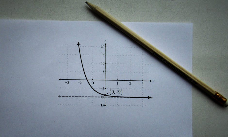
Photo by Sergey Meshkov on Pexels

Exponential functions have distinct shapes. They either shoot upwards rapidly (growth) or approach zero rapidly (decay). They always pass through the point (0, a) because b^0 = 1, so y = a * 1 = a when x = 0. They also have a horizontal asymptote, usually the x-axis (y=0), meaning the function gets very close to it but never actually touches or crosses it.

Half-Life and Doubling Time

Photo by Moose Photos on Pexels

These are special cases of exponential decay and growth, respectively.
* Half-life: The time it takes for a quantity to reduce to half its initial value.
* Doubling time: The time it takes for a quantity to double its initial value.

graph TD
    A["Initial Amount ('a')"] --> B{{"Determine Growth/Decay Factor ('b')"}};
    B -- "If Rate 'r' is Growth" --> C["b = 1 + r"];
    B -- "If Rate 'r' is Decay" --> D["b = 1 - r"];
    C --> E["Exponential Growth (b > 1)"];
    D --> F["Exponential Decay (0 < b < 1)"];
    E --> G["Function: y = a * b^x"];
    F --> G;
    G --> H["Predict Future Value ('y')"];

3. Worked Example

Let's say you invest $1,000 in an account that earns 7% interest compounded annually. How much will you have after 10 years?

1. Identify a (initial amount): a = $1,000
2. Identify r (growth rate): r = 7% = 0.07
3. Calculate b (growth factor): Since it's growth, b = 1 + r = 1 + 0.07 = 1.07
4. Identify x (number of periods): x = 10 years
5. Write the equation: y = 1000 * (1.07)^10
6. Calculate y:
   y = 1000 * 1.96715...
y = $1967.15

So, after 10 years, you'd have approximately $1,967.15.

4. Key Takeaways

• Exponential functions model consistent percentage change over time.
• The base b determines growth (b > 1) or decay (0 < b < 1).
• The starting value is always a when x = 0.
• Exponential growth increases rapidly, while exponential decay approaches zero rapidly.
• Half-life and doubling time are specific applications of exponential decay and growth.

Common mistakes to avoid:
- Confusing adding a fixed amount (linear) with multiplying by a fixed factor (exponential).
- Using r directly as b instead of 1 + r or 1 - r.
- Forgetting to convert percentage rates to decimals (e.g., 5% becomes 0.05).
- Assuming a negative x value means y will be negative (it won't; it just means going backward in time).

5. Now Try It

You bought a new car for $25,000. It depreciates (loses value) by 12% each year. Write an exponential function to model its value, and then calculate what the car will be worth after 5 years. What does success look like? You'll have an equation of the form y = a * b^x and a single dollar value for the car's worth after 5 years.