Curve Sketching and Graphical Analysis

TL;DR

Curve sketching is about understanding a function's behavior and features without plotting every point. You'll use calculus tools like derivatives to identify critical points, concavity, and asymptotes. Putting these pieces together helps you visualize the graph accurately.

1. The Mental Model

Think of curve sketching as being a detective for a function. You're gathering clues (from its equation and derivatives) about where it's going up or down, how it's bending, and if it has any invisible boundaries. Your goal is to build a complete picture from these clues.

2. The Core Material

Curve sketching involves a systematic approach to analyze a function and its derivatives to understand its shape.

a. Domain and Intercepts

Photo by Markus Winkler on Pexels

First, figure out where the function is defined (its domain). Are there any values of x that make the function undefined (like division by zero or square roots of negative numbers)?
Next, find the intercepts:
* y-intercept: Set x = 0 and solve for y.
* x-intercepts: Set y = 0 and solve for x. These are often called roots.

b. Asymptotes

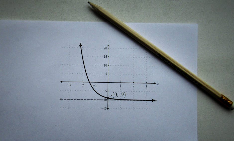
Photo by Sergey Meshkov on Pexels

Asymptotes are lines that the graph approaches but never quite touches (or crosses at infinity).
* Vertical Asymptotes (VA): Look for x-values where the denominator is zero but the numerator is not.
* Horizontal Asymptotes (HA): Examine the limit of the function as x approaches positive or negative infinity.
* If $\lim_{x \to \pm \infty} f(x) = L$ (a finite number), then $y=L$ is a HA.
* Slant/Oblique Asymptotes (SA): If the degree of the numerator is exactly one greater than the degree of the denominator, you might have a slant asymptote. Use polynomial long division to find it: $f(x) = (\text{quotient}) + (\text{remainder}/\text{denominator})$. The SA is $y = \text{quotient}$.

c. First Derivative Test: Increasing/Decreasing Intervals and Local Extrema

Photo by Rafael Minguet Delgado on Pexels

The first derivative, $f'(x)$, tells you about the function's slope.
* Find critical points by setting $f'(x) = 0$ or finding where $f'(x)$ is undefined.
* Test intervals around these critical points:
* If $f'(x) > 0$, the function is increasing.
* If $f'(x) < 0$, the function is decreasing.
* Local Extrema:
* If $f'(x)$ changes from positive to negative, you have a local maximum.
* If $f'(x)$ changes from negative to positive, you have a local minimum.

d. Second Derivative Test: Concavity and Inflection Points

Photo by Sergey Meshkov on Pexels

The second derivative, $f''(x)$, tells you about the function's curvature.
* Find potential inflection points by setting $f''(x) = 0$ or finding where $f''(x)$ is undefined.
* Test intervals around these points:
* If $f''(x) > 0$, the function is concave up (like a cup).
* If $f''(x) < 0$, the function is concave down (like a frown).
* Inflection Points: Occur where $f''(x)$ changes sign.

Here’s a flowchart to help organize your steps:

graph TD
    A["Start: Analyze Function f(x)"] --> B["1. Domain & Intercepts"];
    B --> C["2. Asymptotes (VA, HA, SA)"];
    C --> D["3. Find f'(x)"];
    D --> E["Identify Critical Points (f'(x)=0 or undefined)"];
    E --> F{"Sign of f'(x)?"};
    F -- "+: Increasing" --> G["Local Max/Min"];
    F -- "-: Decreasing" --> G;
    G --> H["4. Find f''(x)"];
    H --> I["Identify Potential Inflection Points (f''(x)=0 or undefined)"];
    I --> J{"Sign of f''(x)?"};
    J -- "+: Concave Up" --> K["Inflection Points"];
    J -- "-: Concave Down" --> K;
    K --> L["5. Sketch the Graph (Plot key points & use features)"];
    L --> M["End"];

e. Symmetry (Optional but Helpful)

• Even function: $f(-x) = f(x)$ (symmetric about the y-axis).
• Odd function: $f(-x) = -f(x)$ (symmetric about the origin).

3. Worked Example

Let's sketch $f(x) = \frac{x}{x^2+1}$.

1. Domain: $x^2+1$ is never zero, so the domain is $(-\infty, \infty)$.
2. Intercepts:
   • y-intercept: $f(0) = \frac{0}{0^2+1} = 0$. So, $(0,0)$.
   • x-intercept: $f(x)=0 \implies x=0$. So, $(0,0)$.
3. Asymptotes:
   • Vertical: None, as denominator is never zero.
   • Horizontal: $\lim_{x \to \pm \infty} \frac{x}{x^2+1} = 0$. So, $y=0$ is a HA.
   • Slant: None, degree of numerator (1) is not one greater than denominator (2).
4. First Derivative:
   $f'(x) = \frac{(1)(x^2+1) - (x)(2x)}{(x^2+1)^2} = \frac{x^2+1-2x^2}{(x^2+1)^2} = \frac{1-x^2}{(x^2+1)^2}$
   Critical points: $f'(x)=0 \implies 1-x^2=0 \implies x=\pm 1$.
   • Test $x=-2$: $f'(-2) = \frac{1-(-2)^2}{( (-2)^2+1)^2} = \frac{1-4}{25} = -\frac{3}{25} < 0$ (decreasing)
   • Test $x=0$: $f'(0) = \frac{1-0^2}{(0^2+1)^2} = \frac{1}{1} = 1 > 0$ (increasing)
   • Test $x=2$: $f'(2) = \frac{1-2^2}{(2^2+1)^2} = \frac{1-4}{25} = -\frac{3}{25} < 0$ (decreasing)
     Local minimum at $x=-1$: $f(-1) = \frac{-1}{(-1)^2+1} = -\frac{1}{2}$. Point: $(-1, -1/2)$.
     Local maximum at $x=1$: $f(1) = \frac{1}{1^2+1} = \frac{1}{2}$. Point: $(1, 1/2)$.
     Increasing on $(-1, 1)$. Decreasing on $(-\infty, -1)$ and $(1, \infty)$.
5. Second Derivative:
   $f''(x) = \frac{(-2x)(x^2+1)^2 - (1-x^2)(2(x^2+1)(2x))}{(x^2+1)^4}$
   $f''(x) = \frac{-2x(x^2+1) - 4x(1-x^2)}{(x^2+1)^3}$ (factor out $x^2+1$)
   $f''(x) = \frac{-2x^3-2x - 4x+4x^3}{(x^2+1)^3} = \frac{2x^3-6x}{(x^2+1)^3} = \frac{2x(x^2-3)}{(x^2+1)^3}$
   Potential inflection points: $f''(x)=0 \implies 2x(x^2-3)=0 \implies x=0, x=\pm \sqrt{3}$.
   • Test $x=-2$: $f''(-2) = \frac{2(-2)((-2)^2-3)}{((_2)^2+1)^3} = \frac{-4(1)}{125} < 0$ (concave down)
   • Test $x=-1$: $f''(-1) = \frac{2(-1)((-1)^2-3)}{((-1)^2+1)^3} = \frac{-2(-2)}{8} > 0$ (concave up)
   • Test $x=1$: $f''(1) = \frac{2(1)(1^2-3)}{(1^2+1)^3} = \frac{2(-2)}{8} < 0$ (concave down)
   • Test $x=2$: $f''(2) = \frac{2(2)(2^2-3)}{(2^2+1)^3} = \frac{4(1)}{125} > 0$ (concave up)
     Inflection points at $x=0, \sqrt{3}, -\sqrt{3}$.
     $f(0)=0$, $f(\sqrt{3}) = \frac{\sqrt{3}}{(\sqrt{3})^2+1} = \frac{\sqrt{3}}{4}$, $f(-\sqrt{3}) = -\frac{\sqrt{3}}{4}$.
     Points: $(0,0)$, $(\sqrt{3}, \sqrt{3}/4)$, $(-\sqrt{3}, -\sqrt{3}/4)$.

Now, you'd plot these points: $(0,0)$, $(-1, -1/2)$, $(1, 1/2)$, $(\sqrt{3}, \sqrt{3}/4)$, $(-\sqrt{3}, -\sqrt{3}/4)$. Draw the horizontal asymptote $y=0$. Then connect the points respecting the increasing/decreasing and concavity intervals.

4. Key Takeaways

• Systematic approach: Always follow the same steps to ensure you don't miss any critical features.
• First derivative for slope: $f'(x)$ tells you where the function goes up (increasing) or down (decreasing).
• Second derivative for curvature: $f''(x)$ tells you how the function bends (concave up or down).
• Critical points and extrema: Maxima and minima occur where $f'(x)=0$ or is undefined.
• Inflection points: These are where