Advanced Probability Applications

TL;DR

You'll learn to use various probability formulas and concepts together to solve complex real-world problems. This involves understanding conditional probability, permutations, combinations, and how to apply them in scenarios like decision-making or risk assessment. The key is breaking down big problems into smaller, manageable probability calculations.

1. The Mental Model

Think of advanced probability as a toolkit. You have different tools (formulas and concepts) and you need to figure out which ones to use and in what order to fix a complex problem, like diagnosing a car issue or predicting game outcomes.

2. The Core Material

When problems get tricky, you often need to combine several probability ideas. You're moving beyond simple single-event probabilities to situations where multiple events occur, influence each other, or where the order matters.

Conditional Probability (Revisited)

Photo by DS stories on Pexels

Remember conditional probability? $P(A|B)$ is the probability of event A happening given that event B has already happened. The formula is $P(A|B) = P(A \cap B) / P(B)$. This is super important when events aren't independent.

Bayes' Theorem

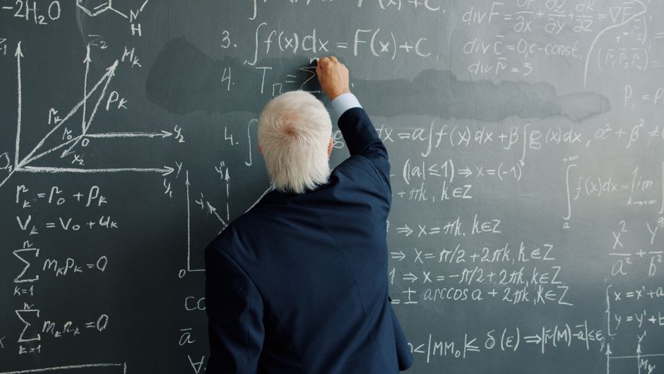
Photo by Vitaly Gariev on Pexels

Bayes' Theorem is a powerful extension of conditional probability, especially useful when you want to update your beliefs about an event after new evidence comes to light. It allows you to reverse the conditional probability. If you know $P(B|A)$, you can find $P(A|B)$.

$P(A|B) = [P(B|A) * P(A)] / P(B)$

Where:
* $P(A|B)$ is the posterior probability: the probability of A given B.
* $P(B|A)$ is the likelihood: the probability of B given A.
* $P(A)$ is the prior probability: the initial probability of A.
* $P(B)$ is the marginal probability: the probability of B.

Often, $P(B)$ can be expanded using the law of total probability: $P(B) = P(B|A)P(A) + P(B|A')P(A')$, where $A'$ is the complement of A.

Permutations and Combinations in Probability

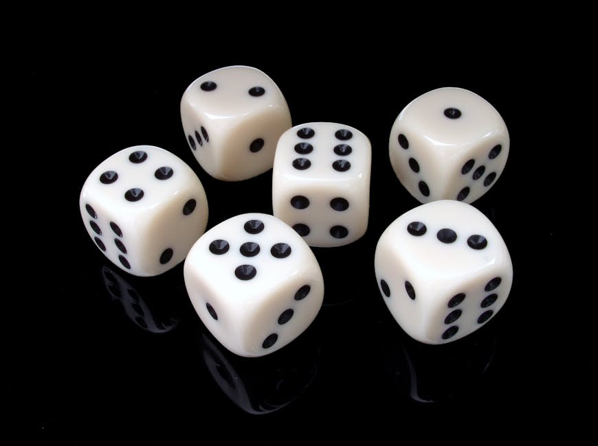
Photo by Pixabay on Pexels

When counting outcomes for probability, sometimes the order matters (permutations), and sometimes it doesn't (combinations).

• Permutations ($P(n, k)$ or $_nP_k$): Used when the order of selection is important. For example, arranging people in a line, or selecting a president and a vice-president. The formula is $P(n, k) = n! / (n-k)!$.
• Combinations ($C(n, k)$ or $_nC_k$): Used when the order of selection does not matter. For example, picking a committee, or choosing lottery numbers. The formula is $C(n, k) = n! / (k!(n-k)!)$.

You'll use these to calculate the number of favourable outcomes and the total number of possible outcomes to find probabilities.

Tree Diagrams for Visualizing Outcomes

Photo by Google DeepMind on Pexels

Tree diagrams are excellent for visualizing sequences of events and their probabilities, especially when dealing with conditional probabilities. Each branch represents an outcome, and you multiply probabilities along branches to find the probability of a sequence of events.

graph TD
    A["Start"] --> B{"Event 1"};
    B --> C["Outcome 1.1 (P=0.6)"];
    B --> D["Outcome 1.2 (P=0.4)"];
    C --> E["Event 2 (given 1.1)"];
    D --> F["Event 2 (given 1.2)"];
    E --> G["Outcome 2.1 (P=0.7)"];
    E --> H["Outcome 2.2 (P=0.3)"];
    F --> I["Outcome 2.3 (P=0.2)"];
    F --> J["Outcome 2.4 (P=0.8)"];

Probability Distributions (Briefly)

Sometimes, your outcomes aren't just "yes/no" but can take on a range of values. This leads to probability distributions. You've probably touched on discrete ones like the Binomial Distribution (for a fixed number of independent trials with two outcomes) or the Geometric Distribution (for the number of trials until the first success). Understanding when to apply these is key. For advanced problems, you might need to determine if a scenario fits one of these common distributions to calculate probabilities efficiently.

3. Worked Example

Let's consider a company that manufactures light bulbs. 2% of the bulbs produced are defective. There's a quality control test that correctly identifies a defective bulb 95% of the time (true positive rate). However, it also incorrectly flags a good bulb as defective 10% of the time (false positive rate). If a bulb is flagged as defective by the test, what's the actual probability that it is truly defective?

Let:
* $D$ = Bulb is defective ($P(D) = 0.02$)
* $D'$ = Bulb is not defective ($P(D') = 1 - 0.02 = 0.98$)
* $F$ = Test flags the bulb as defective

We are given:
* $P(F|D) = 0.95$ (Probability of flagging, given it's defective)
* $P(F|D') = 0.10$ (Probability of flagging, given it's not defective - false positive)

We want to find $P(D|F)$ (Probability that a bulb is defective, given it was flagged).

Using Bayes' Theorem: $P(D|F) = [P(F|D) * P(D)] / P(F)$

First, we need to find $P(F)$, the overall probability of a bulb being flagged. We can use the law of total probability:
$P(F) = P(F|D)P(D) + P(F|D')P(D')$
$P(F) = (0.95)(0.02) + (0.10)(0.98)$
$P(F) = 0.019 + 0.098$
$P(F) = 0.117$

Now, substitute back into Bayes' Theorem:
$P(D|F) = (0.95 * 0.02) / 0.117$
$P(D|F) = 0.019 / 0.117$
$P(D|F) \approx 0.1624$

So, if a bulb is flagged as defective, there's only about a 16.24% chance that it's actually defective. This is much lower than the 95% accuracy rate of the test when the bulb is actually defective, highlighting the importance of Bayes' Theorem in understanding real-world scenarios with low base rates.

4. Key Takeaways

• Always clearly define your events and known probabilities before attempting calculations.
• Conditional probability is fundamental for understanding how events influence each other.
• Bayes' Theorem is crucial for updating probabilities based on new evidence, especially when you need to reverse a conditional probability.
• Use permutations when the order of elements is important, and combinations when it's not, especially for counting outcomes.
• Tree diagrams help visualize sequences of events and multiply probabilities along paths for complex scenarios.
• Recognize when a problem fits a common probability distribution (like Binomial or Geometric) to simplify calculations.

Common Mistakes to Avoid

• Confusing $P(A|B)$ with $P(B|A)$; they are rarely the same.
• Incorrectly applying permutation or combination formulas by mixing up when order matters.
• Forgetting to account for all possible pathways in a tree diagram when calculating total probabilities.
• Assuming events are independent when they are not, leading to incorrect multiplication of probabilities.

5. Now Try It

Imagine a small town where 15% of the population has a rare medical condition. A new diagnostic test is developed. The test has a 90% chance of correctly identifying someone with the condition (true positive rate) and a 5% chance of incorrectly identifying someone without the condition (false positive rate). If a randomly selected person from the town tests positive, what is the probability that they actually have the medical condition?

What to do:
1. Define the events clearly (e.g., $C$ = has condition, $T$ = tests positive).
2. Write down all the probabilities you are given.
3. Use Bayes' Theorem to calculate the required conditional probability.

What success looks like:
You should arrive at a single probability value, expressed as a decimal or percentage, showing the actual chance of having the condition given a positive test result. This value will likely be different from both the 90% true positive rate and the 15% prevalence rate.