Introduction to Geotechnical Engineering and Soil Properties
From the Make notes on soil lab in construction curriculum
TL;DR
Geotechnical engineering is about predicting how soil will behave under a building, road, or slope before you build on it. You'll learn the basic phase relationships (weight, volume, air, water, solids) that every soil lab test relies on. You'll also learn how to classify soil and why that classification drives every foundation decision afterward.
1. The Mental Model
Soil is not one material — it's a mix of solid grains, water, and air, and the proportions of those three things control almost everything: strength, compressibility, drainage. A geotechnical lab doesn't guess these proportions; it measures them directly with weights and volumes. Every formula you'll meet is just accounting — tracking where the mass and volume of a soil sample actually went. If you remember the phase diagram, you can rebuild almost every soil formula from scratch.
2. The Core Material
2.1 The Three-Phase System — the foundation of everything

Photo by Mehmet Turgut Kirkgoz on Pexels
Picture a chunk of soil sitting in a jar. It has three "phases":
- Solids — the actual mineral grains (sand, silt, clay particles)
- Water — fills some of the gaps between grains
- Air — fills whatever gaps the water doesn't
The gaps themselves (water + air together) are called the voids. We draw this as a simple block diagram, splitting volume on one side and mass on the other:
flowchart TB
    subgraph Volume
        Va["Air (Va)"]
        Vw["Water (Vw)"]
        Vs["Solids (Vs)"]
    end
    subgraph Mass
        Ma["Air mass ≈ 0 (Ma)"]
        Mw["Water mass (Mw)"]
        Ms["Solids mass (Ms)"]
    end
    Va --- Ma
    Vw --- Mw
    Vs --- Ms
From this single picture, every core soil property is just a ratio:
Void ratio — voids compared to solids:
$$e = \frac{V_v}{V_s} = \frac{V_a + V_w}{V_s}$$
Porosity — voids compared to the whole sample:
$$n = \frac{V_v}{V} = \frac{e}{1+e}$$
Water content (moisture content) — the single most common lab measurement, mass of water over mass of solids:
$$w = \frac{M_w}{M_s} \times 100\%$$
Degree of saturation — how full the voids are with water (0% = bone dry, 100% = fully saturated):
$$S = \frac{V_w}{V_v} \times 100\%$$
Specific gravity of solids — how much denser the mineral grains are than water (usually 2.65–2.75 for most soils):
$$G_s = \frac{\rho_s}{\rho_w}$$
These five numbers aren't independent — once you know any three of them (plus $G_s$), you can solve for the rest algebraically. That's exactly what a lab report does: measure a couple of things directly (mass, volume, oven-dried mass) and derive the rest.
Unit weight (bulk density, in force per volume) comes from total mass over total volume:
$$\gamma = \frac{W}{V} = \frac{(M_s + M_w) \cdot g}{V}$$
And a very useful relationship ties unit weight to void ratio, water content, and specific gravity directly:
$$\gamma = \frac{G_s (1+w)}{1+e} \gamma_w$$
This equation is your workhorse — most soil lab problems boil down to plugging into this one formula or rearranging it.
2.2 Index Properties — Atterberg Limits and Soil Classification
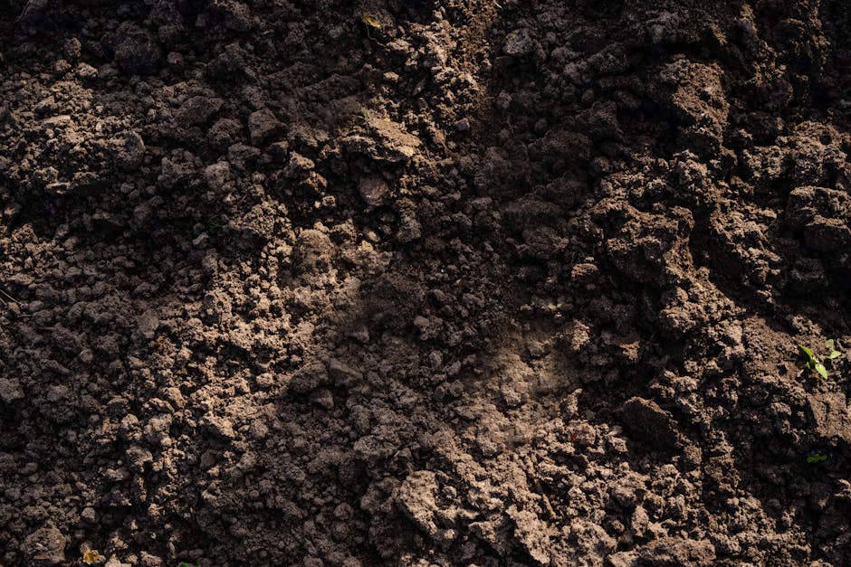
Photo by Atlantic Ambience on Pexels
Phase relationships tell you what's in the soil. Index properties tell you how the soil behaves, especially fine-grained soils like clay and silt.
Atterberg Limits describe how a soil's consistency changes with water content:
- Liquid Limit (LL) — the water content at which soil transitions from a liquid-like paste to a plastic solid. Measured with the Casagrande cup: you cut a groove in wet soil, drop the cup repeatedly, and record the water content at which the groove closes after 25 blows.
- Plastic Limit (PL) — the water content at which the soil stops being plastic and starts crumbling. Measured by rolling the soil into a 3 mm thread until it just starts to crack.
- Shrinkage Limit (SL) — the water content below which further drying causes no further volume change.
From LL and PL, we get the Plasticity Index, which tells you the range of water content over which the soil stays plastic (moldable):
$$PI = LL - PL$$
A high PI (say, 40%) means a soil can absorb a lot of water while staying workable — typical of expansive clays that swell and shrink dramatically with seasons. A low PI (say, 5%) means the soil quickly turns from solid to liquid — more typical of silts, which are notoriously unstable when wet.
Why this matters in construction: PI directly predicts swelling potential. Soils with PI > 20% are flagged for expansive soil problems — they can heave foundations by inches as they wet and dry seasonally. This is one of the most common causes of cracked slabs in residential construction.
2.3 Soil Classification — USCS

Photo by Anna Shvets on Pexels
The Unified Soil Classification System (USCS) is the common language engineers use to describe soil in reports, drawings, and specs. It splits soil first by grain size, then by plasticity:
flowchart TD
    A["Soil sample"] -->|More than 50% passes No. 200 sieve| B["Fine-grained soil"]
    A -->|50% or more retained on No. 200 sieve| C["Coarse-grained soil"]
    B -->|Plot on Plasticity Chart| D{"Above A-line and PI > 7?"}
    D -->|Yes| E["CL / CH — Clay"]
    D -->|No| F["ML / MH — Silt"]
    C -->|More gravel than sand| G["Gravel (G)"]
    C -->|More sand than gravel| H["Sand (S)"]
    G --> I{"Well or poorly graded? Fines content?"}
    H --> I
    I -->|Clean, well graded| J["GW / SW"]
    I -->|Clean, poorly graded| K["GP / SP"]
    I -->|Has fines, plastic| L["GC / SC"]
    I -->|Has fines, non-plastic| M["GM / SM"]
The No. 200 sieve has openings of 0.075 mm — the standard dividing line between "coarse" (gravel/sand, you can see individual grains) and "fine" (silt/clay, grains invisible to the naked eye). This single sieve test decides which branch of the whole classification tree you're on.
Grain size distribution for coarse soils is summarized by two numbers:
Coefficient of uniformity — how spread out the grain sizes are:
$$C_u = \frac{D_{60}}{D_{10}}$$
Coefficient of curvature — checks the shape of the grading curve isn't skewed oddly:
$$C_c = \frac{(D_{30})^2}{D_{10} \times D_{60}}$$
Here $D_{60}$, $D_{30}$, $D_{10}$ are the grain sizes at which 60%, 30%, and 10% of the sample (by weight) is finer. A "well-graded" sand (SW) needs $C_u \geq 6$ and $C_c$ between 1 and 3 — meaning it has a good mix of particle sizes that pack together densely, giving better bearing capacity. A "poorly-graded" sand (SP) is mostly one size — lots of voids, weaker, more permeable.
3. Worked Example
A lab technician runs a standard moisture-density test on a soil sample and reports the following raw data:
- Mass of moist soil + container: 185.4 g
- Mass of oven-dried soil + container: 162.1 g
- Mass of empty container: 32.0 g
- Volume of the moist soil sample (measured by displacement): 85 cm³
- Specific gravity of solids, $G_s = 2.70$
Step 1 — find the water content.
Mass of water: $M_w = 185.4 - 162.1 = 23.3$ g
Mass of dry solids: $M_s = 162.1 - 32.0 = 130.1$ g
$$w = \frac{23.3}{130.1} \times 100\% = 17.9\%$$
Step 2 — find the bulk (total) unit weight.
Total mass of soil (no container): $M = M_s + M_w = 130.1 + 23.3 = 153.4$ g
Bulk density: $\rho = \frac{153.4 \text{ g}}{85 \text{ cm}^3} = 1.805 \text{ g/cm}^3 = 1805 \text{ kg/m}^3$
In unit weight terms: $\gamma = \rho \times g = 1805 \times 9.81 = 17{,}703 \text{ N/m}^3 \approx 17.7 \text{ kN/m}^3$
Step 3 — back out the void ratio using the master equation.
We know $\gamma = 17.7$ kN/m³, $w = 0.179$, $G_s = 2.70$, and $\gamma_w = 9.81$ kN/m³. Rearranging:
$$\gamma = \frac{G_s(1+w)}{1+e}\gamma_w \implies 1+e = \frac{G_s(1+w)\gamma_w}{\gamma}$$
$$1+e = \frac{2.70 \times 1.179 \times 9.81}{17.7} = \frac{31.23}{17.7} = 1.765$$
$$e = 0.765$$
Step 4 — find porosity and degree of saturation.
$$n = \frac{e}{1+e} = \frac{0.765}{1.765} = 0.433 \;(43.3\%)$$
For degree of saturation, first find $V_v = n \times V = 0.433 \times 85 = 36.8 \text{ cm}^3$. Volume of water: $V_w = M_w / \rho_w = 23.3 / 1.0 = 23.3 \text{ cm}^3$.
$$S = \frac{23.3}{36.8} \times 100\% = 63.3\%$$
So this sample is 17.9% water by weight, has 43% of its volume as voids, and those voids are only about 63% full of water — meaning there's still trapped air. This single data set (two masses, one volume, one $G_s$) let us derive five different engineering properties — exactly the kind of calculation a soil mechanics lab report demands.
4. Key Takeaways
4.1 Most Important Concepts

Photo by Roxanne Minnish on Pexels
- Soil is a three-phase system — solids, water, air — and almost every formula is just a ratio between these.
- Water content (w) is the cheapest, most common test — oven-dry a sample, compare wet vs dry mass, done.
- Void ratio (e) and porosity (n) measure the same thing (empty space) but relative to different denominators (solids vs total volume) — know which one a formula wants.
- Atterberg limits (LL, PL, PI) describe clay/silt behavior, not grain size — critical for predicting swelling and shrinking.
- USCS classification splits soils first by grain size (No. 200 sieve), then by plasticity — this decision determines the letter code (e.g., CL, SW, GP) used on every geotechnical report.
- $C_u$ and $C_c$ describe grading shape for coarse soils — well-graded soils compact better and perform better as structural fill.
- The master equation $\gamma = \dfrac{G_s(1+w)}{1+e}\gamma_w$ connects nearly every phase property — memorize it, and you can derive almost anything else from a lab data sheet.
4.2 Common Misconceptions
- "Void ratio and porosity are the same number." They're related but not equal — $e$ divides by solid volume, $n$ divides by total volume; they only look close at low void ratios.
- "High moisture content always means weak soil." Not necessarily — it depends on soil type; a saturated well-graded gravel can still be very strong, while a dry expansive clay can still fail catastrophically when it gets wet later.
- "Plasticity Index measures grain size." It measures behavior (how much water range keeps the soil moldable), completely independent of the No. 200 sieve test for grain size.
- "Specific gravity of solids changes a lot between soils." It actually stays in a narrow band (2.65–2.75) for most mineral soils — organic soils are the main exception, dropping well below 2.6.
4.3 Compare & Contrast
| Property | What it measures | Typical test method | Units |
|---|---|---|---|
| Water content (w) | Mass of water relative to solids | Oven-drying, mass comparison | % (dimensionless) |
| Void ratio (e) | Volume of voids relative to solids | Calculated from mass + volume data | dimensionless ratio |
| Liquid Limit (LL) | Water content where soil becomes liquid-like | Casagrande groove cup test | % water content |
| Plasticity Index (PI) | Range of water content soil stays plastic | LL − PL (calculated) | % (dimensionless) |
5. Now Try It
Exercise: A soil sample has a moist mass of 220 g and volume of 100 cm³. After oven-drying, its mass is 190 g. Given $G_s = 2.65$:
- Calculate the water content $w$.
- Calculate the bulk unit weight $\gamma$ (in kN/m³, using $\gamma_w = 9.81$ kN/m³).
- Use the master equation to solve for void ratio $e$.
- Calculate porosity $n$ and degree of saturation $S$.
Work through it exactly like the worked example above — find masses of water and solids first, then density, then rearrange the master equation.
Success looks like: you get $w \approx 15.8\%$, $\gamma \approx 21.6$ kN/m³, $e \approx 0.424$, $n \approx 0.298$, and $S \approx 100\%$ (fully saturated) — and you can explain in onesentence why S ≈ 100% makes sense given how little air space is left once the voids are calculated.
Frequently asked about Introduction to Geotechnical Engineering and Soil Properties
Study this next
Get the full Make notes on soil lab in construction curriculum
Clone the complete plan to your dashboard for unlimited AI-generated notes, practice quizzes, and a personalised revision schedule.
Save this course free