Foundations of Physics: Quantities, Measurement, and Data Analysis

TL;DR

Physics relies on accurate measurements and understanding the uncertainties associated with them. You'll use SI units for all quantities and learn how to propagate uncertainties through calculations. Proper data analysis, including graphical methods, helps you extract meaningful conclusions from your experiments.

1. The Mental Model

Think of physics as building a house: you need a solid foundation (units), precise tools (measurements), and a way to account for small imperfections (uncertainties). Without these, your house (experiment) will be shaky.

2. The Core Material

In physics, everything starts with measurement. But measurements are never perfect; they always have some uncertainty. You need to know how to handle these uncertainties and present your data clearly.

SI Units and Conversions

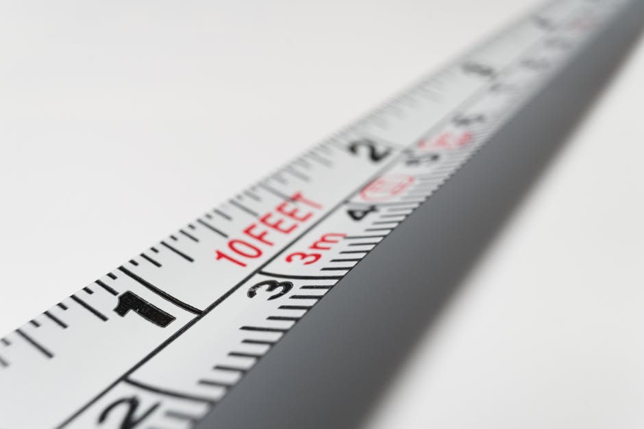
Photo by Pixabay on Pexels

The International System of Units (SI) provides a consistent framework for all physical quantities. You'll always use these in your IB Physics course.

Here are the seven fundamental SI base units:
* Length: meter (m)
* Mass: kilogram (kg)
* Time: second (s)
* Electric current: ampere (A)
* Temperature: kelvin (K)
* Amount of substance: mole (mol)
* Luminous intensity: candela (cd)

All other units are derived units, formed by combining base units (e.g., speed is m/s, force is kg·m/s² which is a Newton, N). You'll often need to convert between different scales using prefixes (e.g., kilo-, milli-, micro-).

Types of Errors and Uncertainties

Photo by Brett Jordan on Pexels

No measurement is perfect. We categorize deviations from the true value as either errors or uncertainties.

• Random Errors: These cause a measured value to deviate unpredictably from the true value. They arise from fluctuations in readings (e.g., slight changes in environmental conditions, difficulty reading scales). You can reduce their impact by taking multiple readings and averaging them. They affect the precision of a measurement.
• Systematic Errors: These consistently shift all measurements in the same direction (either always too high or always too low). They often come from faulty calibration of an instrument, a zero error, or a flawed experimental design. They affect the accuracy of a measurement. They cannot be reduced by repeated measurements.

Uncertainty is a quantification of the doubt about the measurement result. It's not a mistake, but rather a range within which the true value is expected to lie.

Expressing Uncertainty

Photo by https://kaboompics.com/ on Pexels

When you record a measurement, you should always state its uncertainty.

• Absolute Uncertainty: This is the actual range. For a digital instrument, it's usually ± the smallest division or ± half the smallest division. For analog instruments, it's typically ± half the smallest division.
  • Example: A ruler measurement of 2.5 cm might be written as 2.5 ± 0.1 cm.
• Fractional (or Relative) Uncertainty: This is the absolute uncertainty divided by the measured value.
  • Example: For 2.5 ± 0.1 cm, the fractional uncertainty is 0.1/2.5 = 0.04.
• Percentage Uncertainty: This is the fractional uncertainty multiplied by 100%.
  • Example: 0.04 * 100% = 4%.

You should generally only quote uncertainty to one significant figure, and your measured value should be rounded to the same decimal place as its absolute uncertainty.

Propagating Uncertainties

Photo by Mikhail Nilov on Pexels

When you combine measurements through calculations, their uncertainties also combine.

graph TD
    A["Measured Quantities (e.g., A ± ΔA, B ± ΔB)"] --> B{{"Mathematical Operation?"}}
    B --> C1{"Addition or Subtraction: <br> Y = A + B <br> Y = A - B"}
    B --> C2{"Multiplication or Division: <br> Y = A * B <br> Y = A / B"}
    B --> C3{"Powers: <br> Y = A^n"}

    C1 --> D1["Absolute uncertainties add: <br> ΔY = ΔA + ΔB"]
    C2 --> D2["Percentage uncertainties add: <br> %ΔY = %ΔA + %ΔB"]
    C3 --> D3["Percentage uncertainty multiplied by power: <br> %ΔY = n * %ΔA"]

    D1 --> E["Result: Y ± ΔY (absolute uncertainty)"]
    D2 --> E
    D3 --> E

• Addition/Subtraction: When adding or subtracting quantities, you add their absolute uncertainties.
  • If $Y = A + B$ or $Y = A - B$, then $\Delta Y = \Delta A + \Delta B$.
• Multiplication/Division: When multiplying or dividing quantities, you add their percentage uncertainties.
  • If $Y = A \times B$ or $Y = A / B$, then $\frac{\Delta Y}{Y} = \frac{\Delta A}{A} + \frac{\Delta B}{B}$.
• Powers: If a quantity is raised to a power, its percentage uncertainty is multiplied by that power.
  • If $Y = A^n$, then $\frac{\Delta Y}{Y} = n \times \frac{\Delta A}{A}$.

Significant Figures

Significant figures (sig figs) indicate the precision of a measurement.

• Non-zero digits are always significant (e.g., 123 has 3 sig figs).
• Zeros between non-zero digits are significant (e.g., 102 has 3 sig figs).
• Leading zeros (before non-zero digits) are not significant (e.g., 0.0012 has 2 sig figs).
• Trailing zeros (at the end of a number) are significant only if the number contains a decimal point (e.g., 12.00 has 4 sig figs; 1200 has 2 sig figs unless specified).

When performing calculations:
* Multiplication/Division: The result should have the same number of sig figs as the input with the fewest sig figs.
* Addition/Subtraction: The result should have the same number of decimal places as the input with the fewest decimal places.

Graphical Analysis

Graphs are powerful tools to visualize relationships and extract information.

• Plotting points: Use small crosses or circles for data points.
• Error bars: Represent the uncertainty in each measurement on your graph. A vertical error bar shows uncertainty in the y-value; a horizontal error bar shows uncertainty in the x-value.
• Line of best fit: Draw a single, smooth line (straight or curved) that best represents the trend of your data. It doesn't have to pass through every point, but it should have roughly an equal number of points above and below it.
• Gradient and intercepts: For linear graphs, the gradient ($m = \Delta y / \Delta x$) and y-intercept ($c$) are crucial for determining physical constants or relationships ($y = mx + c$).
• Max/min gradients: To determine the uncertainty in the gradient or intercept, draw the steepest and least steep lines that still pass through all error bars. The difference between the best-fit gradient and these max/min gradients gives the uncertainty.

3. Worked Example

Let's say you measure the length ($L$) and width ($W$) of a rectangle to find its area ($A$).

Measurements:
$L = 10.5 \pm 0.1$ cm
$W = 5.2 \pm 0.1$ cm

1. Calculate the area:
   $A = L \times W = 10.5 \text{ cm} \times 5.2 \text{ cm} = 54.6 \text{ cm}^2$

2. Calculate percentage uncertainties for L and W:
   $\% \Delta L = (0.1 \text{ cm} / 10.5 \text{ cm}) \times 100\% \approx 0.952\%$
   $\% \Delta W = (0.1 \text{ cm} / 5.2 \text{ cm}) \times 100\% \approx 1.923\%$

3. Propagate uncertainty for multiplication (add percentage uncertainties):
   $\% \Delta A = \% \Delta L + \% \Delta W = 0.952\% + 1.923\% = 2.875\%$

4. Convert percentage uncertainty back to absolute uncertainty for A:
   $\Delta A = (\% \Delta A / 100) \times A = (2.875 / 100) \times 54.6 \text{ cm}^2 \approx 1.57 \text{ cm}^2$

5. Round uncertainty to one significant figure and the area to the same decimal place:
   $\Delta A \approx 1.6 \text{ cm}^2$ (one sig fig, rounding up)
   $A = 54.6 \text{ cm}^2$ (should be rounded to one decimal place to match uncertainty)
   So, $A = 54.6 \pm 1.6 \text{ cm}^2$

4. Key Takeaways

• Always use SI units and their prefixes; be able to convert between them.
• Distinguish between random errors (precision) and systematic errors (accuracy).
• Quote measurements with their uncertainties, typically to one significant figure for uncertainty and matching decimal places for the value.
• Understand how to propagate uncertainties for addition/subtraction (add absolute) and multiplication/division/powers (add percentage).
• Use error bars on graphs and consider max/min gradients to find uncertainty in calculated values.
• Significant figures matter for representing the precision of your results.

Common Mistakes to Avoid

• Forgetting units or using inconsistent units in calculations.
• Confusing random and systematic errors, or thinking repeated measurements fix systematic errors.
• Adding absolute uncertainties for multiplication/division instead of percentage uncertainties.
• Ignoring significant figure rules, leading to overly precise or imprecise results.
• Drawing lines of best fit that must go through the origin or every point, instead of representing the overall trend.

5. Now Try It

Measure the diameter ($D$) of a coin multiple times using a ruler and a vernier caliper. For each instrument, estimate your absolute uncertainty. Calculate the coin's circumference ($C = \pi D$) for both measurements, including the propagated uncertainty.

What to do:
1. Using a ruler, take 5 measurements of the coin's diameter. Determine the average diameter and its absolute uncertainty (e.g., half the range or standard deviation if you know how).
2. Repeat step 1 using a vernier caliper.
3. For both the ruler and caliper measurements, calculate the circumference $C = \pi D$, propagating the